LAB 11 - Localization using Bayes Filter (on the robot)
Introduction
The aim of this lab is to perform localization utilizing the Bayes Filter on our actual robot. Throughout this lab, only the update step will be used due to the noisiness of the particular robots we are using, which does not contribute to an effective prediction step. Therefore, the update step will be the only one used and is going to be based on the full 360 degree scans of the ToF sensors, similarly to Lab 9 implementation. Ultimately, this lab ought to teach us the main difference between the simulation of the grid localization performed in Python in Lab 10, as compared to the actual real-world system simulation, which is performed in this lab.
Lab Tasks
For this lab, I made a copy of the lab11_sim.ipynb and lab11_real.ipynb provided scripts and places them into the notebooks directory, as well as made a copy of localization_extras.py and places it into the FastRobots-sim-release directory. For the code to be functional with the Bluetooth module, I copied base_ble.py, ble.py, connection.yaml, and cmd_types.py files into the notebooks directory as well.
Localization Simulation
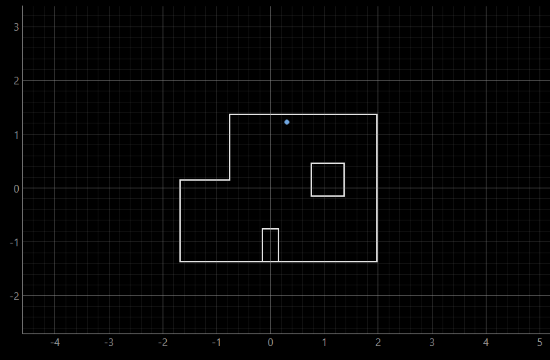
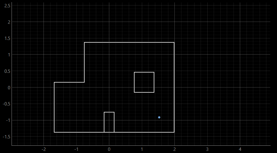
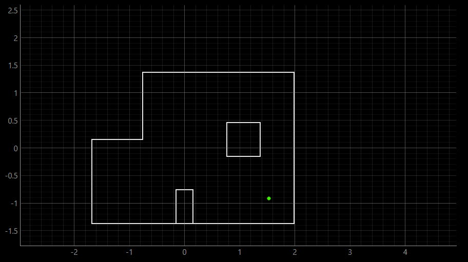
The first proposed task of the lab asked us to perform the Bayes Filter simulation based on the provided lab11_sim.ipynb script, which ought to produce comparable results to what we produced with the Python implementation in Lab 10. The screenshot of the final output can be found below. The green line represents the ground truth, the belief is represented in blue, while the odometry model is represented in red. It can be inferred, similarly to in Lab 10, ground truth and belief are close together, while the odometry model does not effectively and accurately replicate the odometry and belief.
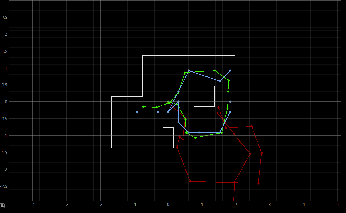 Bayes Filter Algorithm run based on the lab11_sim.ipynb script, indicating odometry model (red), belief (blue), and ground truth (green)
Arduino Implementation
My Arduino code remained very much the same compared to the code provided in Lab 9. The predominant changes to my code were the fact that I set the number of increments (in my code, referred to as steps) to be 18, and the target_yaw, or the angle of increment was changed to be -20 degrees, as opposed to the positive 10 degrees for the angle and 36 steps for the number of increments from Lab 9. Furthermore, I made another change to separate the for loop in which I send my collected data arrays over to Python in a separate case, called SEND_ORIENTATION_DATA. For this reason, the steps variable was instantiated globally, instead of in the main control case, PID_TURN_FULL, since the variable is also called in the SEND_ORIENTATION_DATA case. The code for this case, as well as the primary case PID_TURN_FULL can be seen below.
Full lab 11 Arduino code shown here for reference
case PID_TURN_FULL:
{
    const int steps = 18; // this variable is set globally
    const float yaw_step = -20.0;
    double initial_yaw = 0;
    double target_yaw, current_yaw;
    float error = 0, prev_error = 0, error_sum = 0;
    float dt = 0;
    float pwm = 0, p_term, i_term, d_term;
    unsigned long last_time = millis();

    // Arrays for logging set as global variables
    // double actual_yaw_data[steps];
    // double expected_yaw_data[steps];
    // unsigned long timestamps[steps];
    // int tof_data[steps];

    icm_20948_DMP_data_t data;
    distanceSensor0.startRanging();

    // Obtain the initial yaw
    while (true) {
    myICM.readDMPdataFromFIFO(&data);
        if ((myICM.status == ICM_20948_Stat_Ok || myICM.status == ICM_20948_Stat_FIFOMoreDataAvail) &&
            (data.header & DMP_header_bitmap_Quat6)) {
            double q1 = ((double)data.Quat6.Data.Q1) / 1073741824.0;
            double q2 = ((double)data.Quat6.Data.Q2) / 1073741824.0;
            double q3 = ((double)data.Quat6.Data.Q3) / 1073741824.0;
            double q0 = sqrt(1.0 - ((q1 * q1) + (q2 * q2) + (q3 * q3)));
            double qw = q0, qx = q2, qy = q1, qz = -q3;
            double t3 = 2.0 * (qw * qz + qx * qy);
            double t4 = 1.0 - 2.0 * (qy * qy + qz * qz);
            initial_yaw = atan2(t3, t4) * 180.0 / PI;
            break;
        }
    }

    for (int step = 0; step < steps; step++) {
        target_yaw = initial_yaw + step * yaw_step;
        if (target_yaw > 180) target_yaw -= 360;
        if (target_yaw < -180) target_yaw += 360;

        bool targetReached = false;
        unsigned long turnStartTime = millis();

        // PID Turn Loop
        while (!targetReached && millis() - turnStartTime < 3000) {
            myICM.readDMPdataFromFIFO(&data);
            if ((myICM.status == ICM_20948_Stat_Ok || myICM.status == ICM_20948_Stat_FIFOMoreDataAvail) &&
                (data.header & DMP_header_bitmap_Quat6)) {

            double q1 = ((double)data.Quat6.Data.Q1) / 1073741824.0;
            double q2 = ((double)data.Quat6.Data.Q2) / 1073741824.0;
            double q3 = ((double)data.Quat6.Data.Q3) / 1073741824.0;
            double q0 = sqrt(1.0 - ((q1 * q1) + (q2 * q2) + (q3 * q3)));
            double qw = q0, qx = q2, qy = q1, qz = -q3;
            double t3 = 2.0 * (qw * qz + qx * qy);
            double t4 = 1.0 - 2.0 * (qy * qy + qz * qz);
            current_yaw = atan2(t3, t4) * 180.0 / PI;

            dt = (millis() - last_time) / 1000.0;
            last_time = millis();

            error = current_yaw - target_yaw;
            if (error > 180) error -= 360;
            if (error < -180) error += 360;

            error_sum += error * dt;
            if (error_sum > 150) error_sum = 150;
            if (error_sum < -150) error_sum = -150;

            p_term = Kp * error;
            i_term = Ki * error_sum;
            d_term = Kd * (error - prev_error) / dt;
            pwm = p_term + i_term + d_term;

            prev_error = error;

            if (abs(error) < 2.0) {
                targetReached = true;
                break;
            }

            if (pwm > maxSpeed) pwm = maxSpeed;
            if (pwm < -maxSpeed) pwm = -maxSpeed;

            if (pwm < -100) {
                analogWrite(PIN0, abs(pwm)); analogWrite(PIN1, 0);
                analogWrite(PIN3*1.1, abs(pwm)); analogWrite(PIN2, 0);
            }
            else if (pwm > 100) {
                analogWrite(PIN0, 0); analogWrite(PIN1, abs(pwm));
                analogWrite(PIN3, 0); analogWrite(PIN2*1.1, abs(pwm));
            }
            else {
                analogWrite(PIN0, 0); analogWrite(PIN1, 0);
                analogWrite(PIN3, 0); analogWrite(PIN2, 0);
            }

            delay(10);
            }
        }

        // Stop the motors
        analogWrite(PIN0, 0); analogWrite(PIN1, 0);
        analogWrite(PIN3, 0); analogWrite(PIN2, 0);

        delay(1000); // Pause for 1 second at this angle

        // Get distance
        int distance_tof = 0;
        if (distanceSensor0.checkForDataReady()) {
            distance_tof = distanceSensor0.getDistance();
            distanceSensor0.clearInterrupt();
            distanceSensor0.stopRanging();
            distanceSensor0.startRanging();
            Serial.println(distance_tof);
        }

        // Save data to arrays
        expected_yaw_data[step] = step * 10;
        actual_yaw_data[step] = current_yaw;
        timestamps[step] = millis();
        tof_data[step] = distance_tof;
        }

        Serial.println("A full 360 turn complete.");
        break;
    }
case SEND_ORIENTATION_DATA: {
for (int j = 0; j < steps; j++) {
tx_estring_value.clear();
tx_estring_value.append(expected_yaw_data[j]);
tx_estring_value.append("|");
tx_estring_value.append(actual_yaw_data[j]);
tx_estring_value.append("|");
tx_estring_value.append(timestamps[j]);
tx_estring_value.append("|");
tx_estring_value.append(tof_data[j]);
tx_characteristic_string.writeValue(tx_estring_value.c_str());
}
Serial.println("360-degree PID turn complete, and data is transmitted.");
break;
}
Python Implementation
The initial steps towards Python code were to download and examine the provided lab11_real.ipynb script. Afterwards, I implemented the perform_observation_loop() function in order to sort through the data which is received in arrays from Arduino per every rotation. The function can be found below. A while loop was proposed for when the obtained readings are less than 18, in which case asyncio function was used, as proposed in the Lab 11 manual, which is a coroutine that pauses the execution of current coroutine for 3 seconds, allowing other coroutines to run, as per asyncio.sleep(). Afterwards, the obtained angle readings are assigned to sensor_bearings, while the obtained distance readings are converted to meters from millimeters, and thus assigned to sensor_ranges. The aforementioned case of SEND_ORIENTATION_DATA which obtains the sent arrays of data from Arduino was incorporated into the Python code.
def perform_observation_loop(self, rot_vel=120):
    """Perform the observation loop behavior on the real robot, where the robot does
    a 360 degree turn in place while collecting equidistant (in the angular space) sensor
    readings, with the first sensor reading taken at the robot's current heading.
    The number of sensor readings depends on "observations_count"(=18) defined in world.yaml.

    Keyword arguments:
        rot_vel -- (Optional) Angular Velocity for loop (degrees/second)
                    Do not remove this parameter from the function definition, even if you don't use it.
    Returns:
        sensor_ranges   -- A column numpy array of the range values (meters)
        sensor_bearings -- A column numpy array of the bearings at which the sensor readings were taken (degrees)
                           The bearing values are not used in the Localization module, so you may return a empty numpy array
    """

    global array
    sensor_ranges = np.zeros(18)[...,None];
    sensor_bearings = np.zeros(18)[...,None];
    ble.send_command(CMD.SEND_ORIENTATION_DATA, "")

    while (len(array)<18):
        asyncio.run(asyncio.sleep(3))
    for i in range(18):
        data = array[i].split("|")
        sensor_ranges[i] = float(data[3])/1000
        sensor_bearings[i] = float(data[1])
        print(sensor_ranges[i])
        print(sensor_bearings[i])

    return sensor_ranges, sensor_bearings
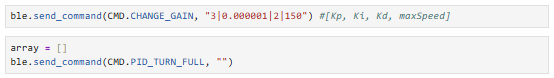
After running the Python portion of the code, as well as connecting via Bluetooth to the Artemis board, I used my code from Lab 5 and 6 in order to change orientation PID control gains, as can be inferred in CHANGE_GAIN case attached below. The optimal gains remained Kp = 3, Ki = 0.000001, and Kd = 2, with maxSpeed variable (from 0-255) being 150, as was determined in the previous labs in order to obtain a tuned rotational movement. Afterwards, the case PID_TURN_FULL was run in order for the robot to rotate. The code for the commands can be found below.
Robot Localization Runs
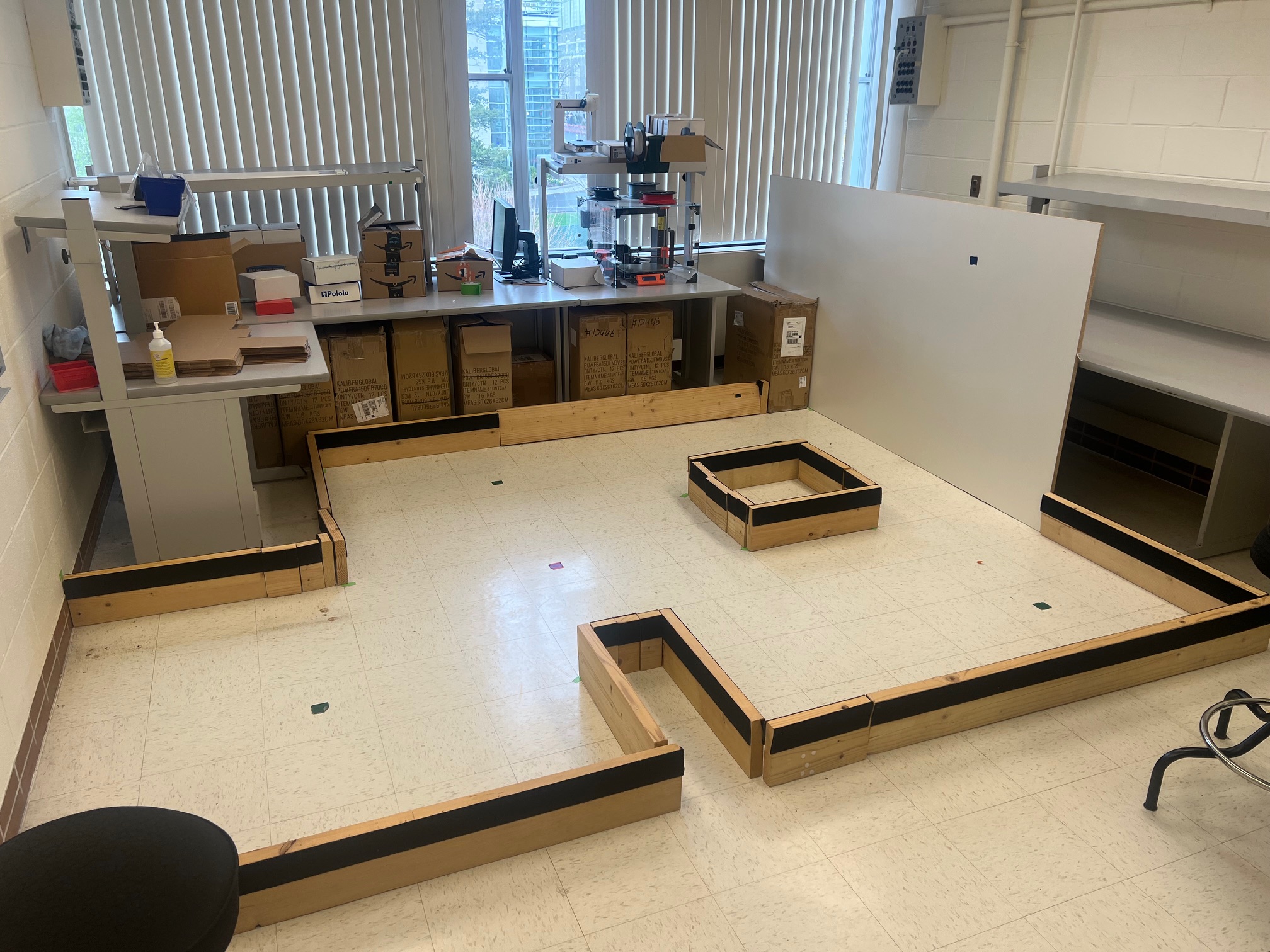
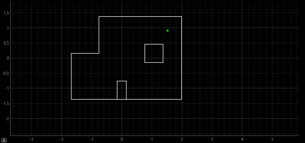
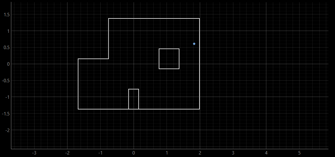
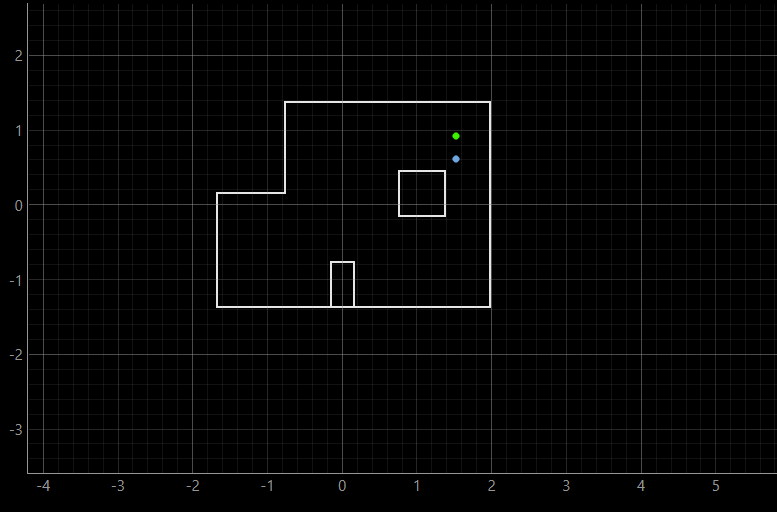
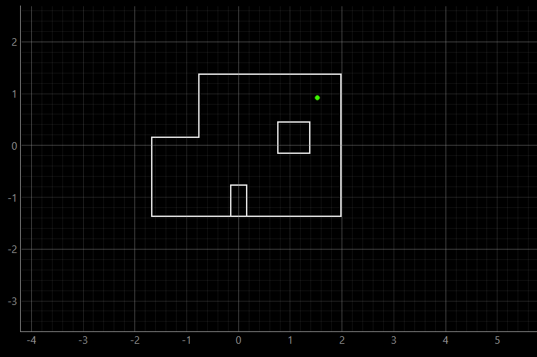
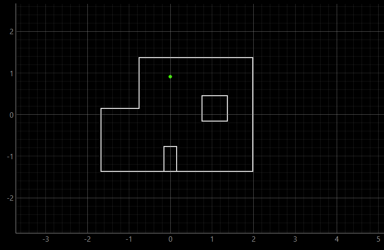
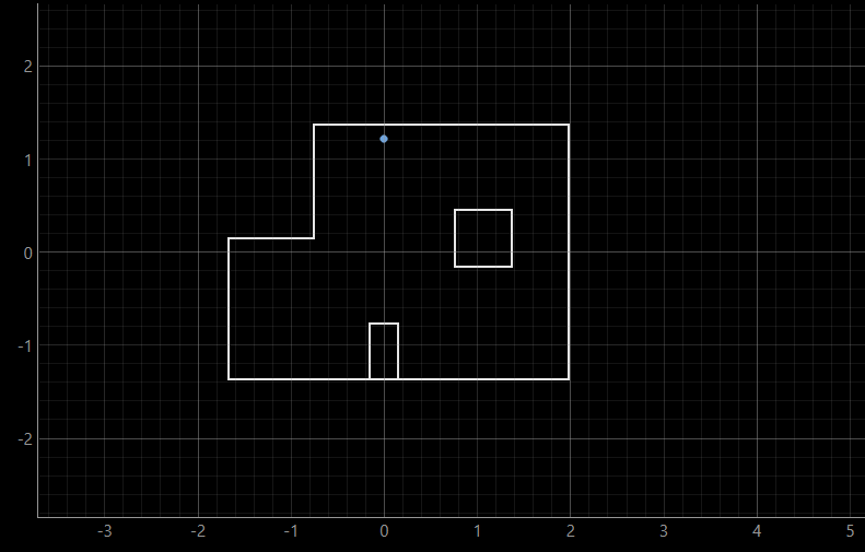
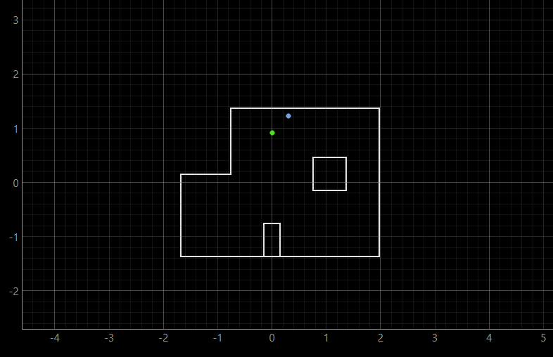
The following task proposed us to rotate the robot about four marked coordinates in the static testing room, its image can be found below (coordinates in feet, (x, y)): (-3,-2), (0, 3), (5, -3), (5, 3). In the plots presented below, ground truth is represented as a green dot, and is the coordinate about which the robot was rotated. The belief was presented as the blue dot. The ToF sensor was oriented to be in positive x direction as its initial position at 0, and would rotate counterclockwise at 20 degrees increments, as aforementioned.
 Testing Static Room
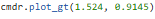
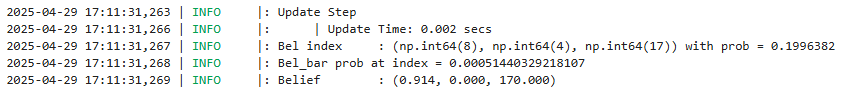
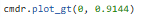
The ground truth was determined to be at the following coordinate represented in meters:
The outputs of the first run can be found below:
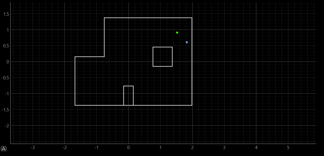
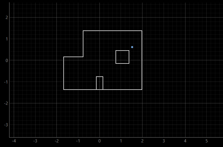
This run, as well as the second run's outputs attached below, yielded belief's positionality slightly below the ground truth. This could be due to slight inconsistency in measured ToF distances, which might have impacted the localization belief.
The results of the second run are as the following:
Finally, the video of the rotation for (5, 3) coordinate can be shown.
(0, 3)The ground truth was determined to be at the following coordinate represented in meters:
The outputs of the first run can be found below:
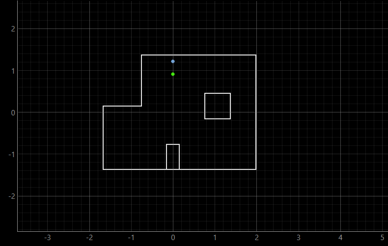
In both of the runs at (0, 3) coordinate, the belief seems to be located higher than the ground truth. I did a couple of runs for this particular point, but they yielded about the same result, with the belief being constantly above ground truth. This is to be expected, considering that this coordinate is bounded by only two walls, which makes the overlap between ground truth and belief harder to achieve. Below we can see another similar output of the (0, 3) coordinate.
The results of the second run are as the following:
Finally, the video of the rotation for (0, 3) coordinate can be shown.
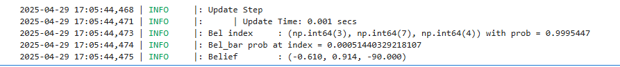
The ground truth was determined to be at the following coordinate represented in meters:

The outputs of the first run can be found below:
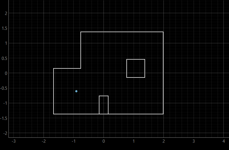
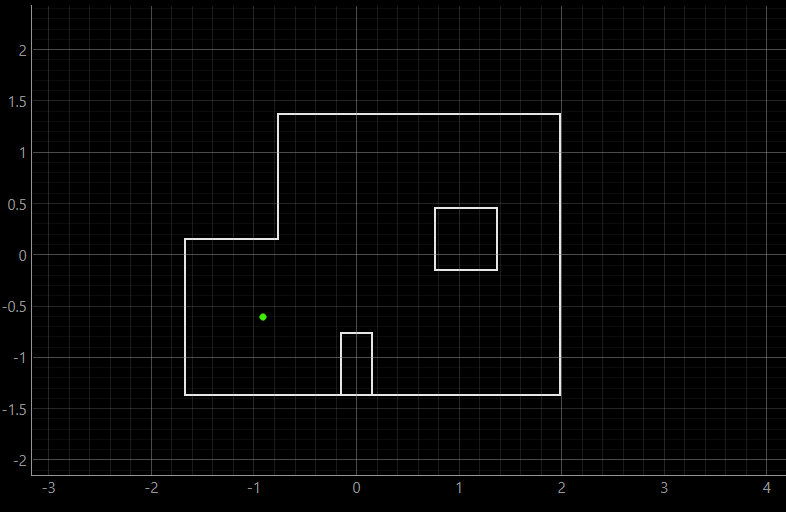
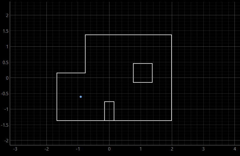
The results of the second run are as the following:
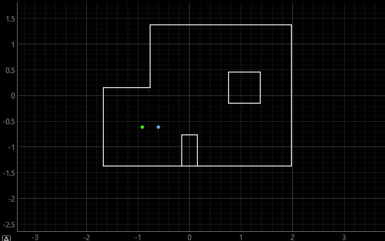
As can be inferred, the ground truth and the belief are at the same point, which can be expected due to the fact that the robot is mostly surrounded by walls from almost all sides, which makes the belief overlab with the ground truth.
Finally, the video of the rotation for (-3, -2) coordinate can be shown.
As can be seen from this run, the belief is slightly dispositioned to the right compared to the ground truth. However, it still maintains a relatively close position to the ground truth.
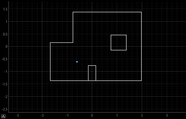
(5, -3)The ground truth was determined to be at the following coordinate represented in meters:

The outputs of the first run can be found below:
As can be inferred from the first run at (5, -3) coordinate, the belief was determined to be at the same point as the ground truth. For both this run, and the outputs of the second run attached below, the ground truth and belief were overlapping. Similarly to the (-3, -2) coordinate, higher accuracy ought to be expected as the robot is surrounded by many walls and a box-shaped obstacle in its view.
The results of the second run are as the following:
Finally, the video of the rotation for (5, -3) coordinate can be shown.
Results Comparison
Based on the presented results, the robot was able to accurately determine the localized pose within a foot of the actual point. Through experimentation, I determined that a lower probability was the result of manipulating the sleep() time in the perform_observation_loop() function, due to changing the time for the ToF sensors to actually obtain the measurements. What is more, I have determined that my robot localizes the best at coordinates (-3,-2), and (5, -3). The reasoning behind this is that both of these coordinates are more bounded by walls and obstacles, and hence the performed measurements are more accurate due to smaller detected distances around the robot. The most inconsistencies I have noticed are in coordinate (5, 3), and that can be due to slight inaccuracies in performed measurements. Generally, the robot was able to perform the localization very well at all points, with slightly higher accuracies with coordinates which are surrounded by more walls and obstacles, and hence result in shorter distance measurements.
Discussion
This lab was very interesting, as it taught us how to utilize Python and Arduino code in order to implement localization on our robots. Furthermore, I enjoy how it built onto what Lab 10 taught us, and expanded it by being able to perform localization on a real-life robot.
Acknowledgements and References
*I referenced TA Mikayla Lahr's website (2024). Special thanks to TA Mikayla for all her help with the lab, and helping me understand the Python implementation better!