LAB 12

Lab Setup

The lab instructions provided us with the following waypoints to navigate throughout the arena. The proposed waypoints are as the following, indicating the start point and the end point, and the screenshot of the arena indicating the path is provided below from the lab handout.

1. (-4, -3)    <--startpoint
2. (-2, -1)
3. (1, -1)
4. (2, -3)
5. (5, -3)
6. (5, -2)
7. (5, 3)
8. (0, 3)
9. (0, 0)      <--endpoint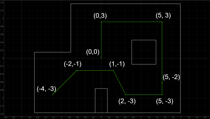

The proposed ideal naviagtion route throughout the arena 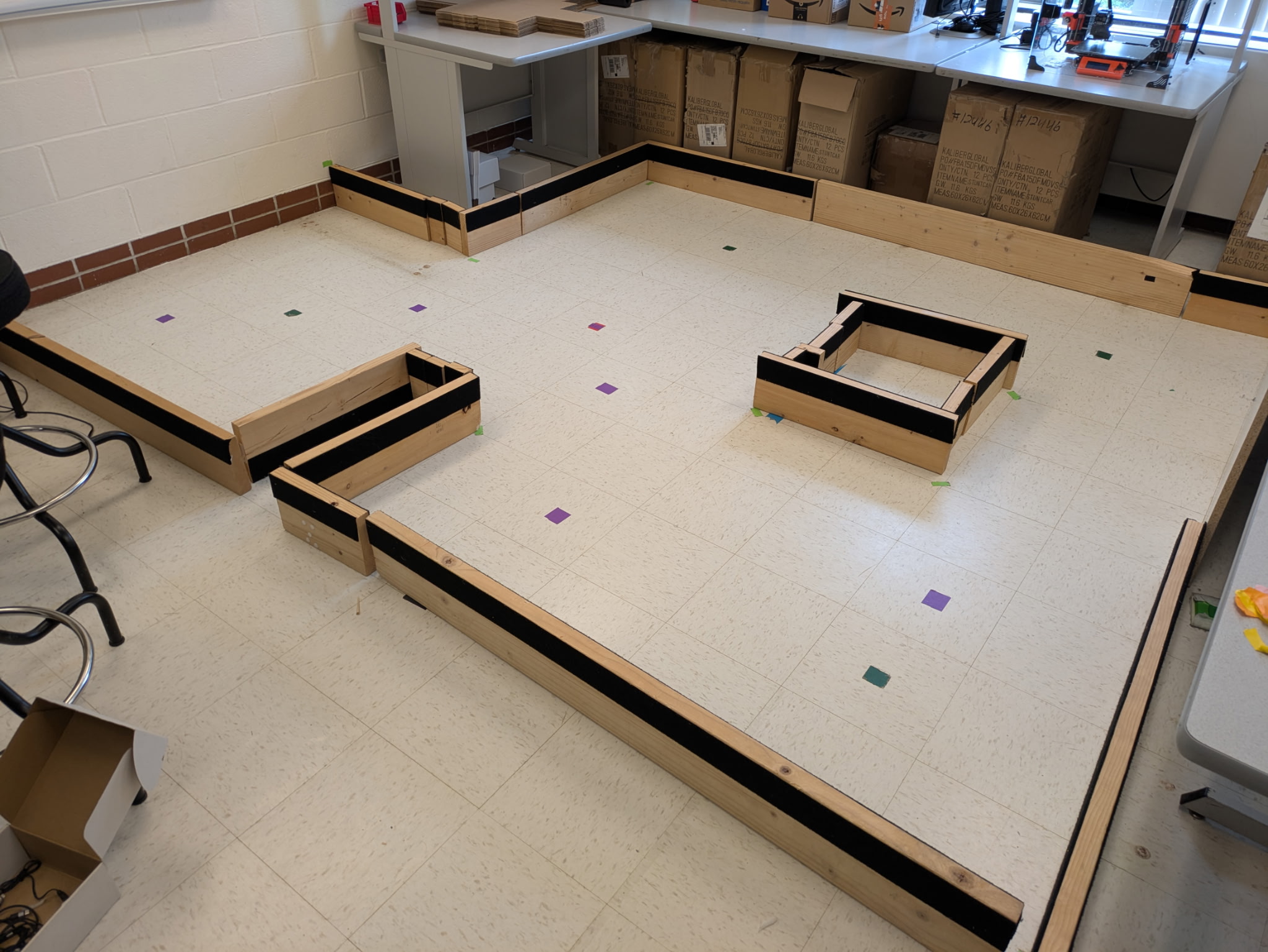The lab arena with the labeled points

Path Planning Design Choices and Procedure

Paul and I wanted to challenge ourselves throughout this lab and perform an entirely closed loop solution. Therefore, our plan was to have the robot calculate the distances it needs to drive from one point to the other, as well as figure out how to retune the angles to move to each of the waypoints. In case of the testing arena being different, our solution should be functional and adaptable to only changing the input map and waypoints. For each of the waypoints, a 5-step solution will be elaborated.

Step 1: Localization

The first step at every point for our robot was to perform localization, and this was performed by utilizing code from Lab 11 on Bayes Filter Localization. The attached code used for the localization step is shown below. This helps the robot determine its position on the map, even in the case of the previous steps being slightly inaccurate.

case PID_TURN_FULL:
{
const int steps = 18; // this variable is set globally
const float yaw_step = -20.0;
double initial_yaw = 0;
double target_yaw, current_yaw;
float error = 0, prev_error = 0, error_sum = 0;
float dt = 0;
float pwm = 0, p_term, i_term, d_term;
unsigned long last_time = millis();

// Arrays for logging set as global variables
// double actual_yaw_data[steps];
// double expected_yaw_data[steps];
// unsigned long timestamps[steps];
// int tof_data[steps];

icm_20948_DMP_data_t data;
distanceSensor0.startRanging();

// Obtain the initial yaw
while (true) {
myICM.readDMPdataFromFIFO(&data);
if ((myICM.status == ICM_20948_Stat_Ok || myICM.status == ICM_20948_Stat_FIFOMoreDataAvail) &&
(data.header & DMP_header_bitmap_Quat6)) {
double q1 = ((double)data.Quat6.Data.Q1) / 1073741824.0;
double q2 = ((double)data.Quat6.Data.Q2) / 1073741824.0;
double q3 = ((double)data.Quat6.Data.Q3) / 1073741824.0;
double q0 = sqrt(1.0 - ((q1 * q1) + (q2 * q2) + (q3 * q3)));
double qw = q0, qx = q2, qy = q1, qz = -q3;
double t3 = 2.0 * (qw * qz + qx * qy);
double t4 = 1.0 - 2.0 * (qy * qy + qz * qz);
initial_yaw = atan2(t3, t4) * 180.0 / PI;
break;
}
}

for (int step = 0; step < steps; step++) {
target_yaw = initial_yaw + step * yaw_step;
if (target_yaw > 180) target_yaw -= 360;
if (target_yaw < -180) target_yaw += 360;

bool targetReached = false;
unsigned long turnStartTime = millis();

// PID Turn Loop
while (!targetReached && millis() - turnStartTime < 3000) {
myICM.readDMPdataFromFIFO(&data);
if ((myICM.status == ICM_20948_Stat_Ok || myICM.status == ICM_20948_Stat_FIFOMoreDataAvail) &&
(data.header & DMP_header_bitmap_Quat6)) {

double q1 = ((double)data.Quat6.Data.Q1) / 1073741824.0;
double q2 = ((double)data.Quat6.Data.Q2) / 1073741824.0;
double q3 = ((double)data.Quat6.Data.Q3) / 1073741824.0;
double q0 = sqrt(1.0 - ((q1 * q1) + (q2 * q2) + (q3 * q3)));
double qw = q0, qx = q2, qy = q1, qz = -q3;
double t3 = 2.0 * (qw * qz + qx * qy);
double t4 = 1.0 - 2.0 * (qy * qy + qz * qz);
current_yaw = atan2(t3, t4) * 180.0 / PI;

dt = (millis() - last_time) / 1000.0;
last_time = millis();

error = current_yaw - target_yaw;
if (error > 180) error -= 360;
if (error < -180) error += 360;

error_sum += error * dt;
if (error_sum > 150) error_sum = 150;
if (error_sum < -150) error_sum = -150;

p_term = Kp * error;
i_term = Ki * error_sum;
d_term = Kd * (error - prev_error) / dt;
pwm = p_term + i_term + d_term;

prev_error = error;

if (abs(error) < 2.0) {
targetReached = true;
break;
}

if (pwm > maxSpeed) pwm = maxSpeed;
if (pwm < -maxSpeed) pwm = -maxSpeed;

if (pwm < -100) {
analogWrite(PIN0, abs(pwm)); analogWrite(PIN1, 0);
analogWrite(PIN3*1.1, abs(pwm)); analogWrite(PIN2, 0);
}
else if (pwm > 100) {
analogWrite(PIN0, 0); analogWrite(PIN1, abs(pwm));
analogWrite(PIN3, 0); analogWrite(PIN2*1.1, abs(pwm));
}
else {
analogWrite(PIN0, 0); analogWrite(PIN1, 0);
analogWrite(PIN3, 0); analogWrite(PIN2, 0);
}

delay(10);
}
}

// Stop the motors
analogWrite(PIN0, 0); analogWrite(PIN1, 0);
analogWrite(PIN3, 0); analogWrite(PIN2, 0);

delay(1000); // Pause for 1 second at this angle

// Get distance
int distance_tof = 0;
if (distanceSensor0.checkForDataReady()) {
distance_tof = distanceSensor0.getDistance();
distanceSensor0.clearInterrupt();
distanceSensor0.stopRanging();
distanceSensor0.startRanging();
Serial.println(distance_tof);
}

// Save data to arrays
expected_yaw_data[step] = step * 10;
actual_yaw_data[step] = current_yaw;
timestamps[step] = millis();
tof_data[step] = distance_tof;
}

Serial.println("A full 360 turn complete.");
break;
} 


case SEND_ORIENTATION_DATA: {
    for (int j = 0; j < steps; j++) {
        tx_estring_value.clear();
        tx_estring_value.append(expected_yaw_data[j]);
        tx_estring_value.append("|");
        tx_estring_value.append(actual_yaw_data[j]);
        tx_estring_value.append("|");
        tx_estring_value.append(timestamps[j]);
        tx_estring_value.append("|");
        tx_estring_value.append(tof_data[j]);
        tx_characteristic_string.writeValue(tx_estring_value.c_str());
        }
        Serial.println("360-degree PID turn complete, and data is transmitted.");
        break;
    }
    

On the Python side for the localization step, the Python code from Lab 11 was also used. The code is incorporated below for reference:

def perform_observation_loop(self, rot_vel=120):
    """Perform the observation loop behavior on the real robot, where the robot does  
    a 360 degree turn in place while collecting equidistant (in the angular space) sensor
    readings, with the first sensor reading taken at the robot's current heading. 
    The number of sensor readings depends on "observations_count"(=18) defined in world.yaml.

    Keyword arguments:
    rot_vel -- (Optional) Angular Velocity for loop (degrees/second)
    Do not remove this parameter from the function definition, even if you don't use it.
    Returns:
    sensor_ranges   -- A column numpy array of the range values (meters)
    sensor_bearings -- A column numpy array of the bearings at which the sensor readings were taken (degrees)
    The bearing values are not used in the Localization module, so you may return a empty numpy array
    """

    global array
    sensor_ranges = np.zeros(18)[...,None];
    sensor_bearings = np.zeros(18)[...,None];
    ble.send_command(CMD.SEND_ORIENTATION_DATA, "")

    while (len(array)<18):
    asyncio.run(asyncio.sleep(3))
    for i in range(18):
    data = array[i].split("|")
    sensor_ranges[i] = float(data[3])/1000
    sensor_bearings[i] = float(data[1])
    print(sensor_ranges[i])
    print(sensor_bearings[i])

    return sensor_ranges, sensor_bearings

For the notification handler, I am using the same code as in the previos labs for obtaining the ToF distances, as well as the yaw data per performing a full turn in order to localize.

//notification handler from the previous labs, including Lab 11
expected_yaw = []
actual_yaw = []
timestamp = []
tof_distance = []
array = []
def lab11_localize(uuid, bytes):
    global array
    s = ble.bytearray_to_string(bytes)
    array.append(ble.bytearray_to_string(bytes)[:])
    if("|" in s):
        sep_notif = s.split("|")
        expected_yaw.append(float(sep_notif[0]))
        actual_yaw.append(float(sep_notif[1]))
        timestamp.append(float(sep_notif[2]))
        tof_distance.append(float(sep_notif[3]))
        
ble.start_notify(ble.uuid['RX_STRING'], lab11_localize)

Step 2: Calculating the Turn Angle

After the localization step, the robot is now aware of its current pose. Our algorithm for calculating the turning angle was for the rovot to use the localized x and y coordinates and hence use them to the angle between the estimated location and its next target waypoint. This can be performed by utilizing the following Python code:

def calcTurnAngle(robotX, robotY, goalX, goalY):
    vecX = goalX - robotX
    vecY = goalY - robotY
    turnAngle = np.arctan2(vecY,vecX)
    return turnAngle

The np.arctan2() math function was used in order to obtain the angle in radians.

Step 3: Turn

After the calculation for finding the correct angle towards the next point is performed, orientation PID control from Lab 6 is performed. This turns the robots to that the ToF sensor faces the waypoint towards which it ought to move next. The code I used for Lab 6 can be found below.

//the following variables are set globally
int i = 0;
unsigned long last_time = millis();
double target_yaw = -30;
double current_yaw = 0;
float dt = 0;
float error_pid;
float pwm;
float error_sum = 0.0;
float p_term = 0.0;
float i_term = 0.0;
float d_term = 0.0;
float old_error;
//end of global variable definitions

case PID_DMP_TURN: {

//DMP quarternion code snippet attached above which stores roll_data[i], pitch_data[i], yaw_data[i], and time_data[i] values
...
// yaw (z-axis rotation)
double t3 = +2.0 * (qw * qz + qx * qy);
double t4 = +1.0 - 2.0 * (qy * qy + qz * qz);
double yaw = atan2(t3, t4) * 180.0 / PI;
yaw_data[i] = yaw;
...
// end of DMP code snippet

dt = (millis()-last_time);
last_time = millis();
current_yaw = yaw;
old_error = error1;
error1 = current_yaw-target_yaw;
error_sum = error_sum + error1*dt;
p_term = Kp * error1;
i_term = Ki * error_sum;
d_term = Kd * (error1 - old_error)/dt;
pwm = p_term + i_term + d_term;

if(pwm > 0)
{
    if(pwm > maxSpeed)
    pwm = maxSpeed;
}
else if(pwm < 0)
{
    if(pwm < -maxSpeed)
    pwm = -maxSpeed;
}
pwm_data[i] = pwm;
    if(pwm < -80) { // needs to be clockwise motion because yaw difference is negative
        analogWrite(PIN0,abs(pwm)); //right backward
        analogWrite(PIN1,0); // right foward
        analogWrite(PIN3,abs(pwm)); //left forward 
        analogWrite(PIN2,0); // left backward
    }
    else if(pwm > 80) // 80 was determined to be the minimum spinning PWM in Lab 4
        { 
        analogWrite(PIN0,0);
        analogWrite(PIN1,abs(pwm));
        analogWrite(PIN3,0);
        analogWrite(PIN2,abs(pwm));
    else{
        analogWrite(PIN0,0);
        analogWrite(PIN1,0);
        analogWrite(PIN3,0);
        analogWrite(PIN2,0);
    }
}
if (myICM.status != ICM_20948_Stat_FIFOMoreDataAvail) // if more data is available then we should read it right away - and not delay
{
delay(10);
}

for (int j = 0; j < i; j++) {
    tx_estring_value.clear();
    tx_estring_value.append(pitch_data[j]);
    tx_estring_value.append("|");
    tx_estring_value.append(roll_data[j]);
    tx_estring_value.append("|");
    tx_estring_value.append(yaw_data[j]);
    tx_estring_value.append("|");
    tx_estring_value.append(time_data[j]);
    tx_estring_value.append("|");
    tx_estring_value.append(pwm_data[j]);
    tx_characteristic_string.writeValue(tx_estring_value.c_str());
    }
Serial.println("PID turning data sent!");
break;
}

Considering that Step 2 of this process calculates the angle through the provided calcTurnAngle() function, I modified my code for tuning the PID control gains to include modifying the target yaw through the send_command() function on the Python side. This enables passing the specific calculated values from the calcTurnAngle() function depending on what the angle calculated for the respective waypoints is much more easily.

Step 4: Calculating distance to move to the next Waypoint

With the turn step, the robot ought to be oriented so that its ToF sensor looks at the wall to which it ought move using linear PID, and stop once it arrives to the next waypoint. In order for this to work, a ray is projected from the robot's front, and the nearest point of intersection between the ray and one of the walls is recorded. We decided to save the coordinates of each of the walls in the arena, by saving them into a numpy array maintaining the form of [x1, y2, x2, y2]. The dimensions can be found below, in meters.

 map = np.array([
    [-1.6764, -1.3716, -1.6764, 0.1524], # [x1, y1. x2. y2]
    [-1.6764, 0.1524, -0.762, 0.1524], 
    [-0.762, 0.1524, -0.762, 1.3716], 
    [-0.762, 1.3716, 1.9812, 1.3716], 
    [1.9812, 1.3716, 1.9812, -1.3716], 
    [1.9812, -1.3716, -1.6764, -1.3716], 
    [-0.1524, -1.3716, -0.1524, -0.762], 
    [-0.1524, -0.762, 0.1524, -0.762], 
    [0.1524, -0.762, 0.1524, -1.3716], 
    [0.762, -0.1524, 0.762, 0.4572], 
    [0.762, 0.4572, 1.3716, 0.4572], 
    [1.3716, 0.4572, 1.3716, -0.1524], 
    [1.3716, -0.1524, 0.762, -0.1524]
    ])

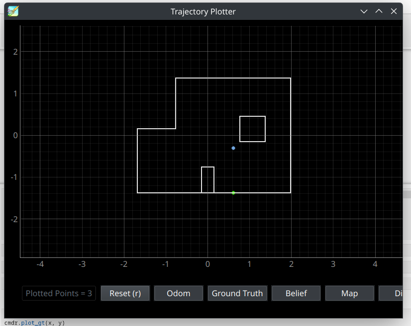
This helps us create a depthPredict() function, which takes in the estimation of robot's pose, along with the coordinates of the map. The function returns x and y coordinates of a single point on the wall at which the ToF sensor is oriented. For instance, as can be seen in Figure () below, the green dot represents the point on the wall, while blue dot represents the robot's pose estimation. The code for this function can be seen below.

def depthPredict(robotX, robotY, robotTheta, robot_map):
    maxRange = 20
    # Define the endpoint of the sensor's line of sight (far away)
    xEnd = robotX + maxRange * np.cos(robotTheta)
    yEnd = robotY + maxRange * np.sin(robotTheta);
    cmdr.plot_odom(xEnd, yEnd) 
    # Initialize minimum depth to a large value
    minDepth = maxRange
    minX = 20
    minY = 20

    # Loop through each wall in the map
    for i in range(len(robot_map)):
        # Extract wall coordinates
        x1 = robot_map[i][0]
        y1 = robot_map[i][1]
        x2 = robot_map[i][2]
        y2 = robot_map[i][3]

        # Check for intersection between sensor line and wall
        [isect, xInt, yInt] = intersectPoint(robotX, robotY, xEnd, yEnd, x1, y1, x2, y2)

        if isect:
            # Calculate distance from sensor to intersection point
            dist = abs(np.sqrt((xInt - robotX)**2 + (yInt - robotY)**2))

            # Update minimum depth if this intersection is closer
            if dist < minDepth:
                minDepth = dist
                minX = xInt
                minY = yInt

    return minX, minY

The following function is crucial in determining the points on the wall in which the ray intersects.

def intersectPoint(x1, y1, x2, y2, x3, y3, x4, y4):
    x = []
    y = []
    ua = []
    
    denom = (y4-y3)*(x2-x1)-(x4-x3)*(y2-y1)
    
    if denom == 0:
        # if denom = 0, lines are parallel
        isect = False
    else:
        ua = ((x4-x3)*(y1-y3) - (y4-y3)*(x1-x3))/denom
        ub = ((x2-x1)*(y1-y3) - (y2-y1)*(x1-x3))/denom
        # if (0 <= ua <= 1) and (0 <= ub <= 1), intersection point lies on line
        # segments
        if ua >= 0 and ub >= 0 and ua <= 1 and ub <= 1:
            isect = True
            x = x1 + ua*(x2-x1)
            y = y1 + ua*(y2-y1)
        else:
            # else, the intersection point lies where the infinite lines
            # intersect, but is not on the line segments
            isect = False
    return isect, x, y

Based on the robot's orientation towards the next waypoint once the turning of the angle is performed, it can be deduced that the next waypoint lies somewhere between the robot's current pose and the point that was calculated on the wall. Hence, the distance from the aforementioned point on the wall to the desired waypoint is the same distance at which we ought to stop the robot's movement to lie on the waypoint. This can be performed with the following code snippet:

def calcStopDist(wallX, wallY, goalX, goalY):
    stopDist = np.sqrt((wallX-goalX)**2 + (wallY - goalY)**2)
    return stopDist*1000 # Converting to mm

Step 5: Moving towards the desired waypoint

The last step of the 5-step process was to send the obtained distance that needs to be performed towards the waypoint to our robot. Upon this, the robot performs linear PID control from Lab 5, but incorporating Kalman Filter from Lab 7 in order to drive towards the wall, and ultimately stop and settle at the waypoint by utilizing Kalman filter. The code I used for this is similar to my Lab 7 code.

case PID_KALMAN: 
{
    //...PID variable instantiation from Lab 5
    float kf_distance;

    Ad  = I + Delta_T * A ;
    Bd = Delta_T * B;
    Cd = C;

    distanceSensor1.startRanging();  //Write configuration bytes to initiate measurement
    Serial.println("Staring Kalman Filter with PID!");
    int t_0 = millis();
    int prev_time = t_0;
    while (!distanceSensor1.checkForDataReady())
    {
        delay(1);
    }
    distance1 =  distanceSensor1.getDistance();
    distanceSensor1.clearInterrupt();
    mu = {(float) distance1, 0.0};
    while ((i < ARRAY_LENGTH && j < ARRAY_LENGTH2) && millis() - t_0 < 5000) {
    time_data[i] = millis();
    if (distanceSensor1.checkForDataReady()) { //ToF sensor data available
        dt = millis() - prev_time;
        prev_time = millis();
        distance1 = distanceSensor1.getDistance();  //Get the result of the measurement from the sensor
        distanceSensor1.clearInterrupt();
        distance_data1[i] = distance1;
        i++;
        y = (float) distance1; //y(0,0) = (float) distance1;
        mu_p = Ad*mu + Bd*u;
        sigma_p = Ad*sigma*~Ad + sigma_u;
        sigma_m = Cd*sigma_p*~Cd + sigma_z;
        kkf_gain = sigma_p*~Cd*Inverse(sigma_m);
        y_m = y-Cd*mu_p;
        mu = mu_p + kkf_gain * y_m;
        sigma = I - kkf_gain*Cd*sigma_p;
        kf_distance = mu(0,0);
        kf_distance = (float) kf_distance;
        if (j < ARRAY_LENGTH2) { 
        kf_distance_array[j] = kf_distance;
        kf_time[j] = millis();
        j++;
        }
        // Start of Control Loop Calculations
        current_dist = distance1;
        distance1 = mu(0,0);
        old_error = error1;
        error1 = current_dist - target_dist; 
        //PID Control from Lab 5
        error_sum = error_sum + (error1 * dt / 1000);
        p_term = Kp * error1;
        i_term = Ki * error_sum;
        d_term = Kd * (error1 - old_error) / dt;
        pwm = p_term + i_term + d_term;
    }
    else{ // ToF sensor data not available, make predictions with Kalman Filter
        mu_p = Ad*mu + Bd*u;
        sigma_p = Ad*sigma*~Ad + sigma_u;
        kf_distance = mu_p(0,0);
        kf_distance = (float) kf_distance;
        mu = mu_p;
        sigma = sigma_p;
        if (j < ARRAY_LENGTH2) { 
        kf_distance_array[j] = kf_distance;
        kf_time[j] = millis();
        j++;
        }
        dt = millis() - prev_time;
        prev_time = millis();
        current_dist = kf_distance;
        old_error = error1;
        error1 = current_dist - target_dist; 
        //PID Control from Lab 5
        error_sum = error_sum + (error1 * dt / 1000);
        p_term = Kp * error1;
        i_term = Ki * error_sum;
        d_term = Kd * (error1 - old_error) / dt;
        pwm = p_term + i_term + d_term;
    }
    // Update motors the same way as in Lab 5
    break;
    }

Final results and Demonstration of Path Planning

The video demonstrating our implementation of path planning around the lab arena can be seen below. Based on the video, I will be covering and describing each of the waypoints individually, the obtained localization data for each of them, as well as discussing difficulties we have faced with tuning our parameters.

As can be inferred from the video, in our proposed path planning solution, there are six waypoints that are being localized out of eight, with the exception of the start waypoint already being the known pose of the robot, and the last waypoint, since once it is reached, we have already completed the navigation through the arena.

Waypoint 1: (-4, -3)

Our robot starts off with its ToF sensor initially being oriented in the direction of positive x-axis, representing the initial yaw value of 0, as in Lab 9 and Lab 11. Considering that there was not a reason to perform localization, as our robot is aware of its pose at the start point and the starting point is always the same, localization is skipped, and the second indicated step of calculating the correct turn angle towards the subsequent waypoint is calculated. The calculated angle is 45 degrees, the robot moves in the counterclockwise direction, and the ToF sensor ends up seeing the following distance on the wall opposite of the ToF sensor, which looks as the following (indicated in green). This helps us move to the next waypoints, while still being oriented and seeing this point on the wall. Using linear PID with Kalman Filter, we move in the direction towards the point we see on the wall, but settle once overlay with the waypoint. The first point is represented in the video in timestamps 0:00-0:28.

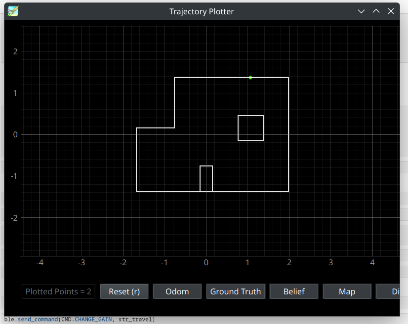The first point's depth prediction indicated in a green dot

Waypoint 2: (-2, -1)

Now that we have moved to the second waypoint, we localize first in order to establish the robot's pose in the arena and confir that it is (-2, -1). The following image shows the localized position of our robot in blue. Even though the robot overshoots the waypoint, the localization was accurate enough for it to still be able to accurately estimate the turn angle towards the third waypoint. The robot then corrects its angle as before, and after performing the aforementioned functions in step 4, sees the point closest to it on the wall it is facing, and uses that to estimate its distance to the next waypoint. The depth prediction point on the wall is reflected in the green plot on the graph below. The second figure indicates the localization update step output, with the indicated probability and belief. The second waypoint is covered in the video under the timestamps of 0:28-1:27.

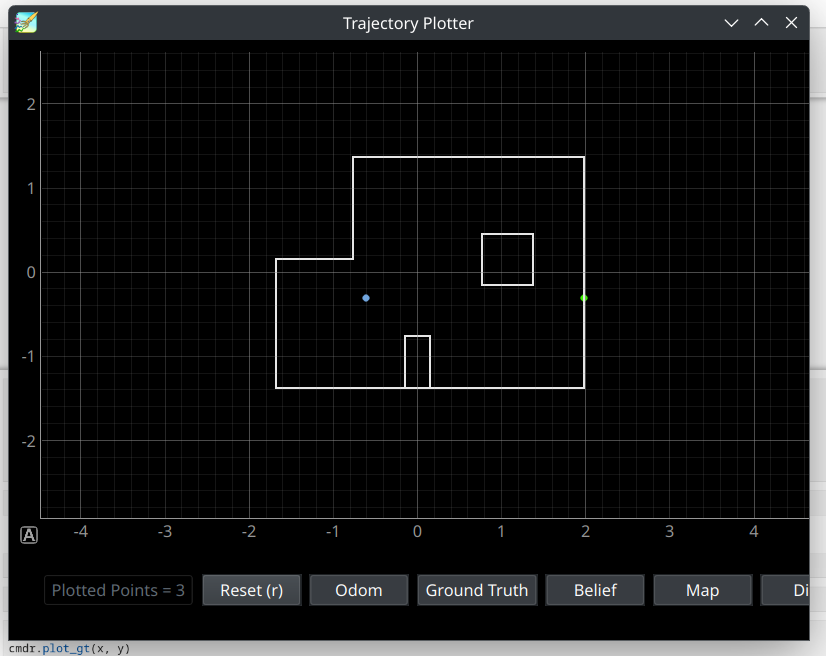The second point's depth prediction indicated in a green dot, and current pose per localization indicated in the blue point.

The second point's depth prediction indicated in a green dot, and current pose per localization indicated in the blue point.

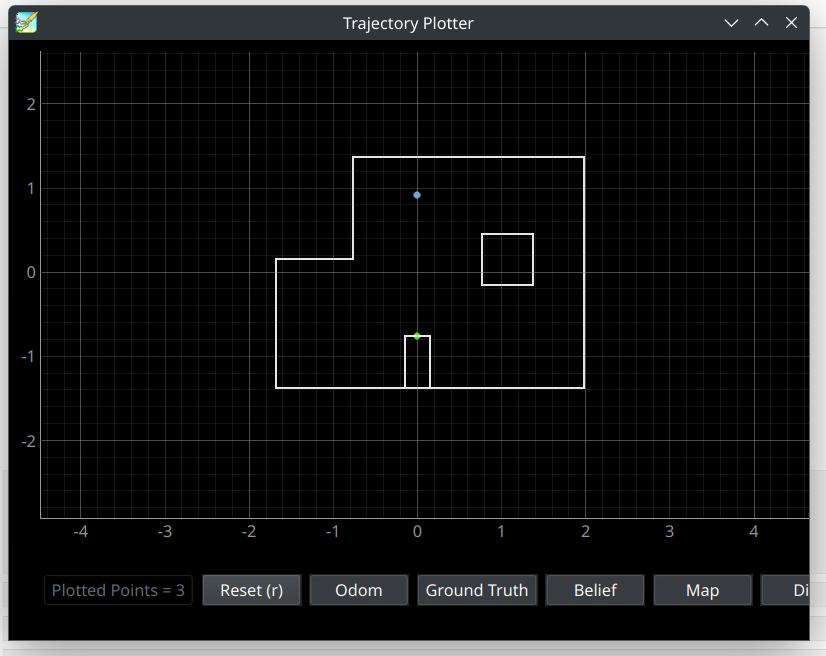
Waypoint 3: (1, -1)

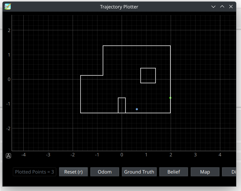
Now that we have moved to the third waypoint, we perform a similar process as with the second waypoint. We localize first in order to establish that the robot's position in the arena is (1, -1). The localization occurred slightly more in the positive x-direction compared to the proposed waypoint, due to a slight overshoot in PID control. What this ultimately meant is that the robot's predicted depth on the wall (indicated in green) is shown to be straight down from the localization result (indicated in blue), indicating that the robot should drive straight down to reach the fourth waypoint. Instead, it should have been under an angle of -63 degrees if the robot localized exactly at (1, -1). The second figure indicates the localization update step output, with the indicated probability and belief. The third waypoint is covered in the video under the timestemps of 1:27-2:35.

The third point's depth prediction indicated in a green dot, and current pose per localization indicated in the blue point.

The third point's depth prediction indicated in a green dot, and current pose per localization indicated in the blue point.

Waypoint 4: (2, -3)

Now that we have moved to the fourth waypoint, we perform a similar process as previously. Considering that the localization for the previous waypoint was slightly inaccurate, the robot drove slightly towards negative x-direction compared to the actual waypoint. The localization reflected in the output being diagonally right and below the actual waypoint. The potentail explanation for this is due to the fact that Bayes Filter's update step (as can be seen from the screenshot below) detected the robot position very close to the wall. Hence, potentially a grid space closer to the wall became the robot's new pose. The fourth waypoint is covered in the video under the timestemps of 2:35-3:34.

The fourth point's depth prediction indicated in a green dot, and current pose per localization indicated in the blue point.

The fourth point's depth prediction indicated in a green dot, and current pose per localization indicated in the blue point.

Waypoint 5: (5, -3)

Now that we have moved to the fifth waypoint, we perform a similar process as previously. What we found interesting is that even though the previous waypoint's localization ended up being slightly incorrect from the fourth waypoint, the robot still managed to move to the fifth waypoint well. This time, the robot settled at a point that is slightly towards right and bottom from the fifth waypoint, which can be reflected in the trajectory plotter results. Even though this was the case, the localized point was in line with the next waypoint well enough for it to move to the next waypoint smoothly. The fifth waypoint is covered in the video under the timestemps of 3:34-4:26.

The fifth point's depth prediction indicated in a green dot, and current pose per localization indicated in the blue point.

The fifth point's depth prediction indicated in a green dot, and current pose per localization indicated in the blue point.

Waypoint 6: (5, -2)

Considering that our localization for waypoints of 5 and 7 performed well for the majority of our trials, and the robot would smoothly drive from waypoint 5 to waypoint 7, we decided to skip localization and planning for waypoint 6. Otherwise, we might have not achieved as smooth of a transition to waypoint 7.

Waypoint 7: (5, 3)

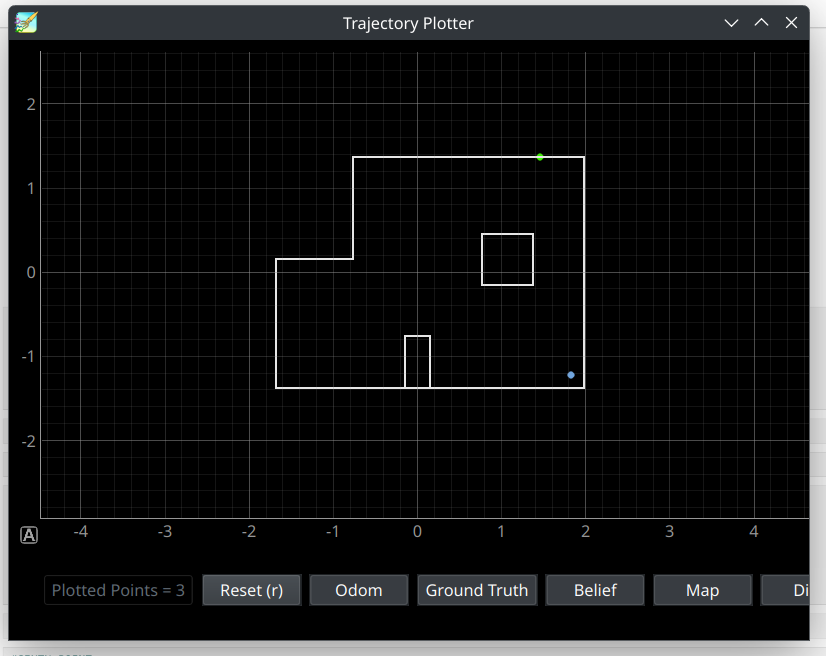
Similarly to fouth and fifth waypoints' localization results, waypoint seven's localization is slightly in the positive x-direction from the actual waypoint's position. However, there were not invariations in the y-direction, so detecting the depth on the wall (indicated in green), which the robot will use to move towards the waypoint, is accurate. The seventh waypoint is covered in the video under the timestemps of 4:34-5:21.

The seventh point's depth prediction indicated in a green dot, and current pose per localization indicated in the blue point.

The seventh point's depth prediction indicated in a green dot, and current pose per localization indicated in the blue point.

Waypoint 8: (0, 3)

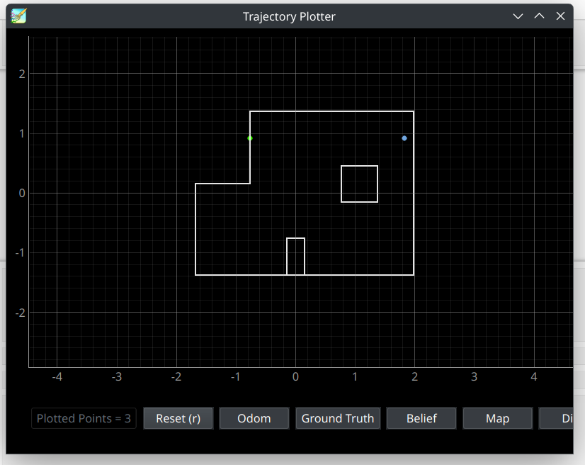
Based on my and Paul's predictions, the robot's movement around this point is slightly impacted by the battery, which is running low based on the video, hence the very well-tuned robot had issues staying in a single spot when localizing. Hence, due to the slight battery issue, the distance towards waypoint eight is slightly underestimated before Bayes Filter localization (indicated in blue) is performed. The robot localizing slightly in the positive x-direction compared to the waypoint (0,3), ended up reflecting in the robot adjusting its angle and driving slightly towards positive x-direction from the waypoint 9 as well (which can be reflected in the green dot on the wall) The eighth waypoint is covered in the video under the timestemps of 5:21-6:39.

The eighth point's depth prediction indicated in a green dot, and current pose per localization indicated in the blue point.

The eighth point's depth prediction indicated in a green dot, and current pose per localization indicated in the blue point.

Waypoint 9: (0, 0)

Since this was the ending waypoint of our path planning journey, there was no need for us to perform localization and planning on this waypoint. The ninth waypoint is covered in the video under the timestamps 6:39-6:59.

Challenges and Issues Faced

Considering that we decided to partner up, Paul and I implemented our Python code for both of our robots, but we decided to run our individual Arduino code from previous labs as the basis for our individual Arduino code portion. Even though the Python code worked successfully on our individual robots, my robot would often struggle with completing and going through the whole arena without disconnecting from Bluetooth. Paul's robot showed higher consistency with the runs, so we decided to dedicate our time into tunning the gains of PID control for his robot instead. This allowed us to utilize our time effectively for performing optimizations.

Another challenge for us was using the Kalman Filter to optimize the robot movement towards a new waypoint better. We, however, realized that we had to retune