LAB 2 - IMU
Introduction:
The aim of this lab was to learn how to adequatelly use the Inertial Measurement Unit, or the IMU. Furthermore, this lab provided me with the knowledge of the accuracy and noise analysis when computing pitch, roll, and yaw of IMU's accelerometer and gyroscope respectively.
Prelab 2: Setup of IMU
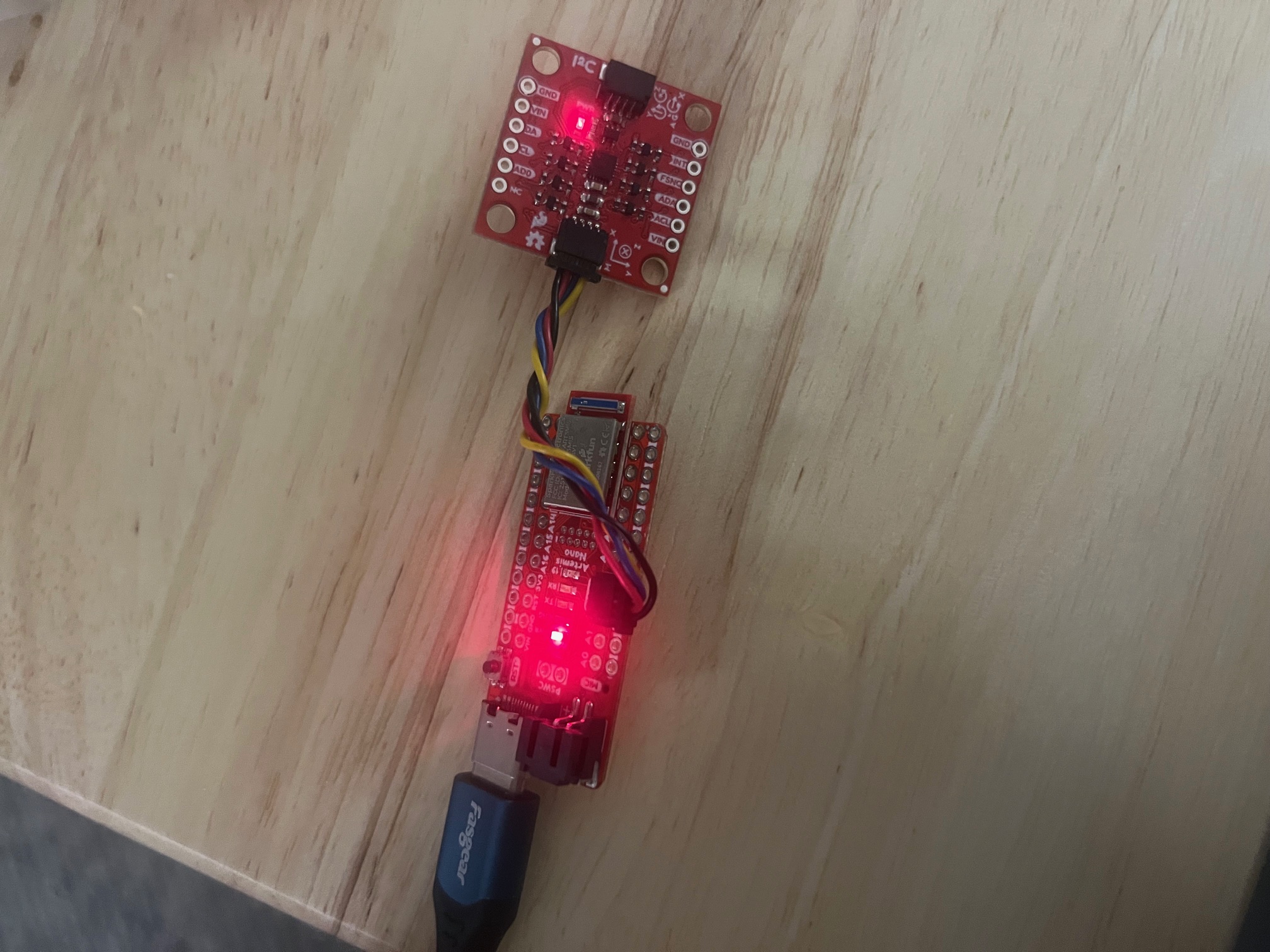
The initial step towards using the IMU was to download the Sparkfun ICM 20948 library which was performed by connecting the IMU device to the Artemis board through the QWIIC connector, as seen in the image below. A significant step towards the very end of the lab was to prepare the RC car by charging the provided 850 mAh batteries.
Lab 2:
IMU example code
The first step was to confirm that the IMU example Arduino code was functional with our IMU device. Hence, SparkFun 9DOF IMU Breakout_ICM 20948_Arduino Library was installed. The outputs observed on the Serial Monitor once the example1_basicscode in the ICM 20948 library was run suggested that there is a variation in accelerometer and gyroscope values once the IMU position was changed.
The provided video displays the change in the output data of the Serial Monitor for accelerometer and gyroscope values dependending on the orientation of the IMU. It can be inferred that the accelerometer measures accelerations relative to the gravitational acceleration (g) direction. On the other hand, the gyroscope detects the change in angle per time unit with regards to the zeroth state at the IMU start. The data of the gyroscope is represented in degrees, hence, the angular rate is integrated over time.
As can be inferred from the video, the provided Example1_Basics code was expanded with the visual in terms of the LED blinking slowly three times. This visual is to indicate that the board is running and has uploaded the code successfully.
AD0_Val Definition
The Ad0_VAL signal is crucial because it represents the last bit of the I2C address for the IMU. This value is set to have the value of 1, due to the fact that we have a single IMU on the I2C bus. If we were to have multiple, the bit would have been jumped on the IMU breakout board in order to have multiple IMUs on the same I2C bus.

Accelerometer
The accelerometer reading require specifications of x, y, and z axes of the coordinate system, which is indicated on the IMU itself. In order to calculate pitch θ and roll Φ, the following equations may be implemented for the Artemis. The equations were incorporated from lecture 4.
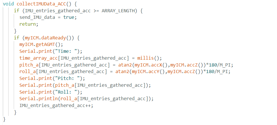
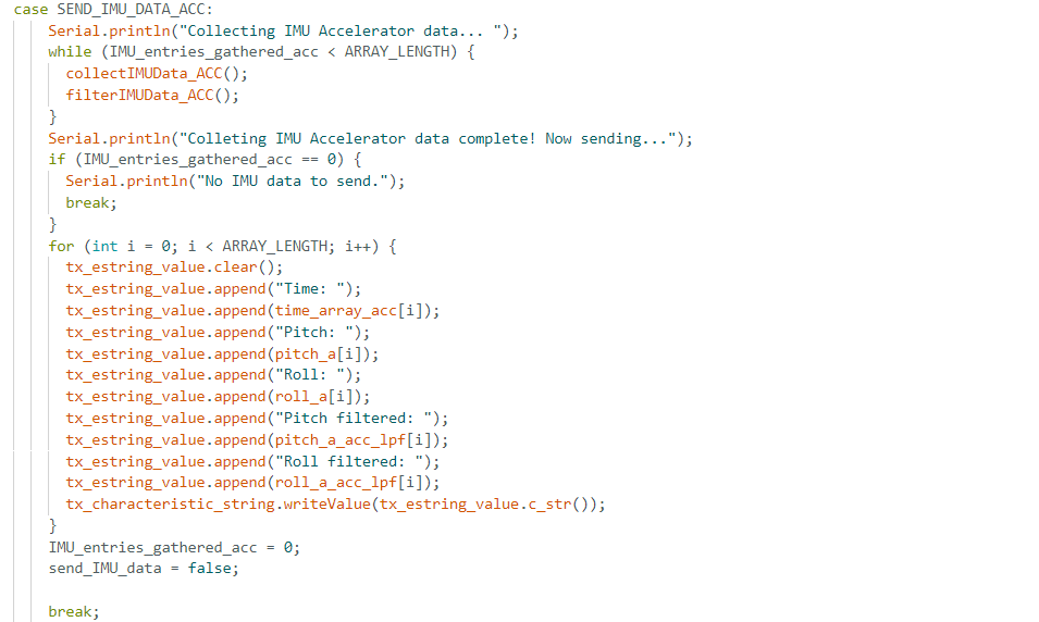
These equations are first incorporated in the Arduino code as in the snippet provided below. As can be seen, I created a function called collectIMUData_ACC() which computes pitch and roll values of the accelerometer while collecting data in real time. Furthermore, pitch, roll, as well as time values are stored in respective arrays of length ARRAY_LENGTH = 2000. The function is called from the SEND_IMU_DATA_ACC case for as long as the number of entries collected is less than the proposed ARRAY_LENGTH.
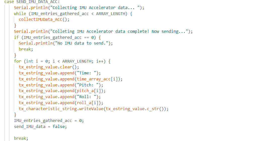
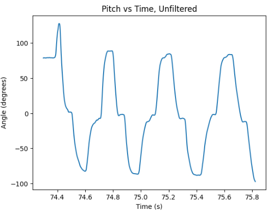
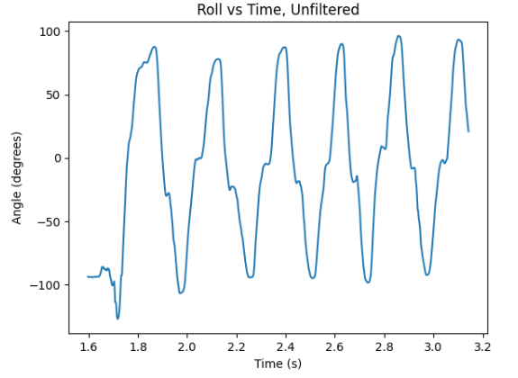
The data is thus sent over through Bluetooth, similarly to lab 1, after which the collected data may be graphed. By oscillating the IMU about the x and y axis as labeled on the device, the following graphs are obtained. The first graph from left to right represents pitch data with respect to time, and the second represents roll data with respect to time of the accelerometer. It can be observed that the IMU is thus able to correctly identify the orientations as learned from class lectures.
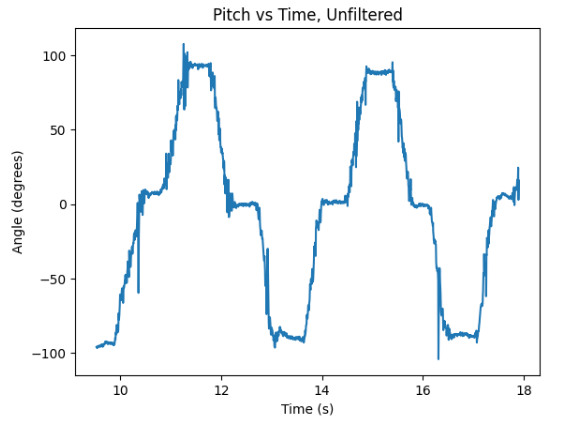
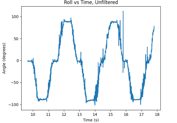
As can be observed, the output for both pitch and roll data display the sequence of {-90, 0, 90} degrees. The graphs were generated by developing a Python script for plotting the data sent from Arduino over time. The results of the accelerometer appear to accurately detect and record the orientation changes, hence the two-point calibration is not necessary. However, the results appear noisy, especially in the regions of switching between orientations of the accelerometer, and thus, a Fourier spectrum might be observed.
Fourier Transform of accelerometer data
The Fourier transform was performed by utilizing SciPy's fft() function in order to detect the periodicity in the signal. As can be observed in the FFT spectrum analysis below, due to the fact that there is significant noise observed for the fact that there was minimal movement while recording pitch and roll data, a low-pass filter ought to be implemented for smoothing out the non-negligible noise.
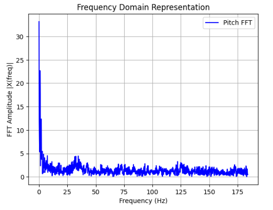
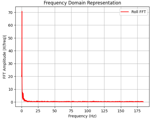
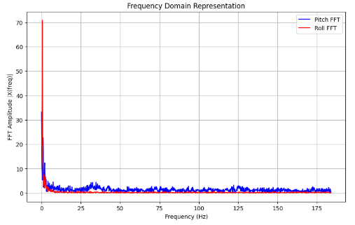
Based on the provided graphs, it can be inferred that the sampling frequency can be estimated to be around 50 Hz, hence I chose the low-pass filter cutoff frequency fcto be about 5 Hz.
Implementation of Low-pass filter
Italic Equations with MathJax
$$ \theta_{lpf}[n] = \alpha \theta_{unfiltered} + (1-\alpha)\theta_{lpf}[n-1] $$
Italic Equations with MathJax
$$ \theta_{lpf}[n-1] = \theta_{lpf}[n] $$
The coefficient α as well as the sampling period T may be calculated through the following formulas:
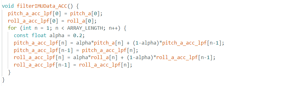
The sampling frequency of the captured IMU data was found to 10 ms per sample. Hence, with the cutoff frequency of about 5 Hz, the value of α ends up being equal to 0.2. Utilizing the aforementioned equations for the implementation of the low-pass filter, the Arduino code ought to be updated as the following:
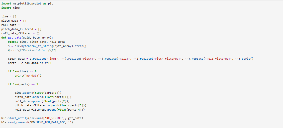
Furthermore, on the Python side, the computation code for with the filter applied was implemented as the following:
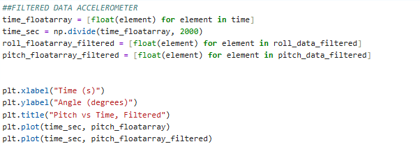
Finally, the applied low-pass filter on the recorded and stored pitch and roll data would be presented as following:
As can be observed from the provided graphs, the low-pass filter (as indicated in orange) is able to significantly reduce the noise in the originally recorded data (as indicated in blue). The noise levels were already minor considering that the accelerometer has an integrated low-pass filter (as is stated in the ICM 20948 datasheet). However, with this implementation of low-pass filter, the noise levels remain negligible and are almost fully reduced.
Gyroscope
As opposed to the accelerometer, the gyroscope is reflected in three leading equations that describe its movement. Each of the equations are integrated over time.
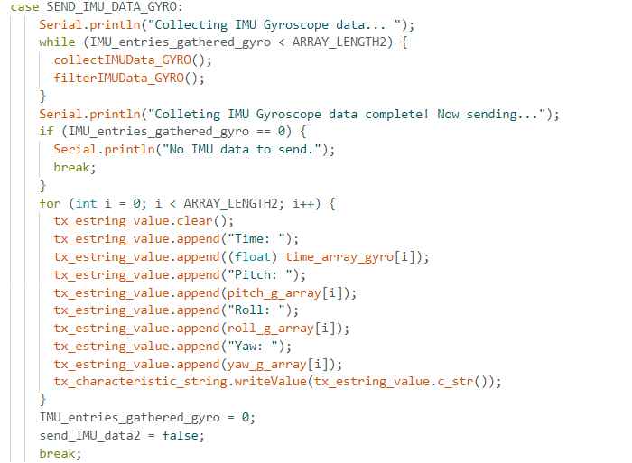
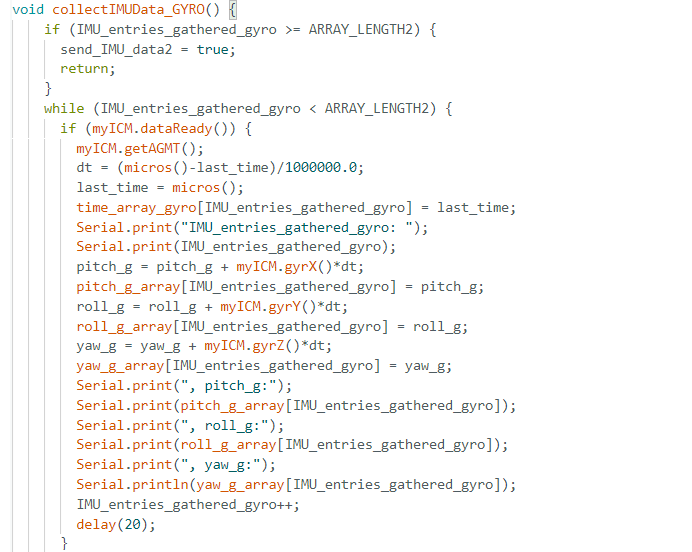
Similarly, to the code for accelerometer, I created a I created a function called collectIMUData_GYRO() which computes pitch, roll, and yaw values of the accelerometer while collecting data in real time. Furthermore, pitch, roll, as well as time values are stored in respective arrays of length ARRAY_LENGTH2 = 2000. The function is called from the SEND_IMU_DATA_GYRO case for as long as the number of entries collected is less than the proposed ARRAY_LENGTH2.
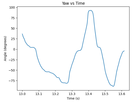
Similarly to testing the accelerometer, I tested the gyroscope by varying {-90, 0, 90} angles for pitch, roll, and yaw respectively. Pitch and roll data were computed unfiltered initially, in order for them to be more easily compared to the accelerometer pitch and roll data. Lastly, yaw data was computed. It could have been observed that pitch and roll data were much less noisy overall compared to the accelerometer's respective data.
Another significant observation while computing the filtered versions of gyroscope's pitch and roll data is that gyroscopre significantly drifts over time, as can be observed below. I decided to compute the gyroscope pitch and roll data as reliably as possible by developing a complimentary filter, which combines the aforementioned definition of accelerometer's RC filter and gyroscope's formulas in order to obtain the following equations. The value of γ represents the coefficient which weighs the relationship between the accelerometer and the gyroscope. Considering the higher accuracy of the accelerometer, the coefficient of γ is set to be 0.8.
Hence, the code implementation on the Arduino side is as following:

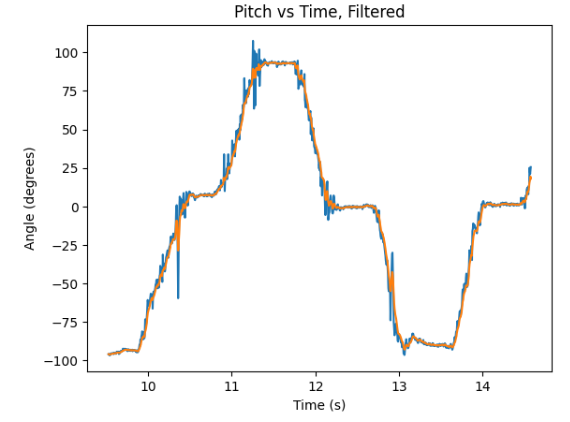
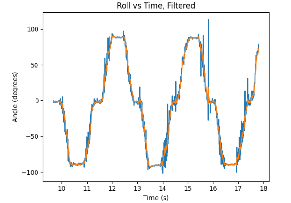
Finally, by rotating the IMU with varying speeds, the filtered accelerometer data was plotted on the same graph as the complementary filter data of the gyroscope, for easier comparison.
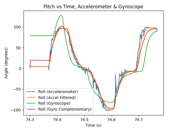
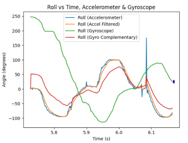
As can be observed, the complementary filter is very accurate with the computation of both pitch and roll data over time, it is able to remain uninfluenced by the detectible drift in data, yet is not influenced by rapid varying and rotating of the IMU. Hence, the complimentary filter is evaluated to be very reliable from the presented graphs. Another observation was that decreasing the sampling frequency ultimately resulted in a greater fluctuation between the measurements of the filtered and unfiltered data. Hence, the sampling rate ought to be high in order to maintain high accuracy in data acquisition.
Sample Data
Timing Analysis and time-stamped arrays
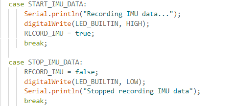
Following the proposed instructions, all the time-consuming and repetitive statements in the main loop have been removed, including all Serial.print() functions, and all the implemented delay() functions. In order to create time-stamped IMU data arrays, a flag RECORD_IMU was instantiated in Arduino cases. Afterwards, GET_IMU_DATA_ACC was called on the Python side in order to determine the computation time or the speed of sampling. This was performed on the ARRAY_LENGTH size of the array, which was previously used in this lab. The code for computation can be found below.
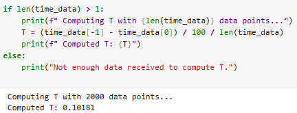
As can be inferred from the provided outputs, the time step T, which represents the speed of data transmission of the data points sent over from Arduino is approximately 0.102.
data storage
In order to compute and store the data for the lab, I stored pitch, roll, and yaw respectively into separate float arrays. This choice ended up aligning with easier manipulation of the data and possibility of easier calculations in the future labs. Each of the float arrays takes up a third of Artemis's 384 kiB of memory. Hence, this corresponds to about 33000 data points. Considering that the sampling rate of the IMU was approximated to be about 220 Hz, this would in theory equate to about 150 seconds to fill the available memory.However, realistically this might not be the case since there are more things occupying the memory, hence the proposed sampling rate would be somewhat smaller in reality.
5s of Data Demonstration
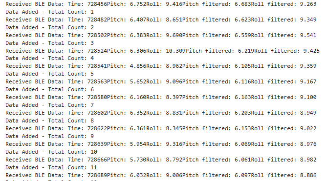
I set the flag indicating that the data collection ought to last for 5 seconds. Furthermore, my array consisted of the GET_IMU_DATA_ACC array, and each of the received arrays had a time stamp indicated.
Record a stunt!
Discussion:
The performed tasks were very insightful and helpful in demonstrating how to properly use the IMU and has set crucial fundamentals for navigating the future labs.