LAB 3 - Time of Flight (ToF)
Introduction:
The aim of this lab was to integrate Time of Flight (ToF) sensors which will be crucial in the ultimate functionality of the car by accurately detecting the surrounding objects.
Prelab 3:
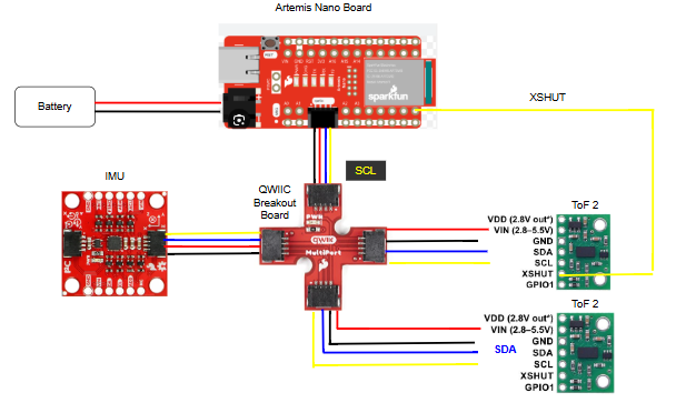
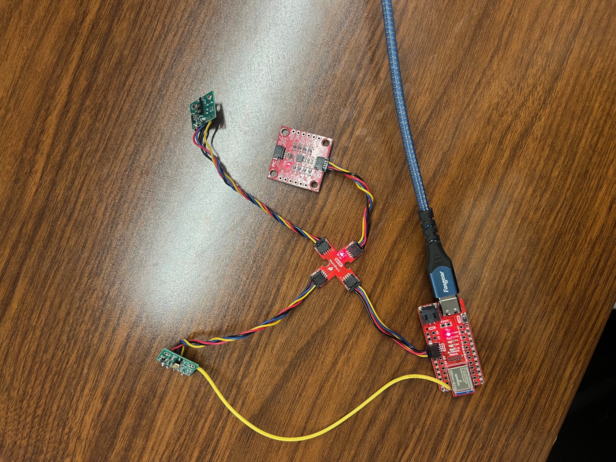
The fundamental step of the prelab was to determine the wiring of the two ToF sensors, as well as how they would integrate with the IMU used in the previous lab. By reading through the datasheet, it was determined that the blue connection indicated on the diagram below represents SDA, and the labeled yellow connection represents SCL. The proposed sensors communicate through I2C, including the IMU from the previous lab, thus the QWIIC breakout board ought to be used establishing the connection among all sensors. The weires connecting from the QWIIC connector are further stripped and soldered onto the two ToF sensors.
Considering that the colour convention of the provided JST connector matched the colour convention of the battery connecting to the Artemis (that is, + terminal connecting to JST connector's red wire, and - terminal of the battery connecting to JST connector's black wire) the connector and the wires feeding into the battery connect as indicated in the diagram above. The connector from the LiPo battery was removed by separating the wires one at a time, and then cutting them individually. The connection between the LiPo battery and the wires was heat shrunk for a secure connection.
Afterwards, SParkFun VL53L1X 4m laser distance sensor library was installed for ToF sensor operation.
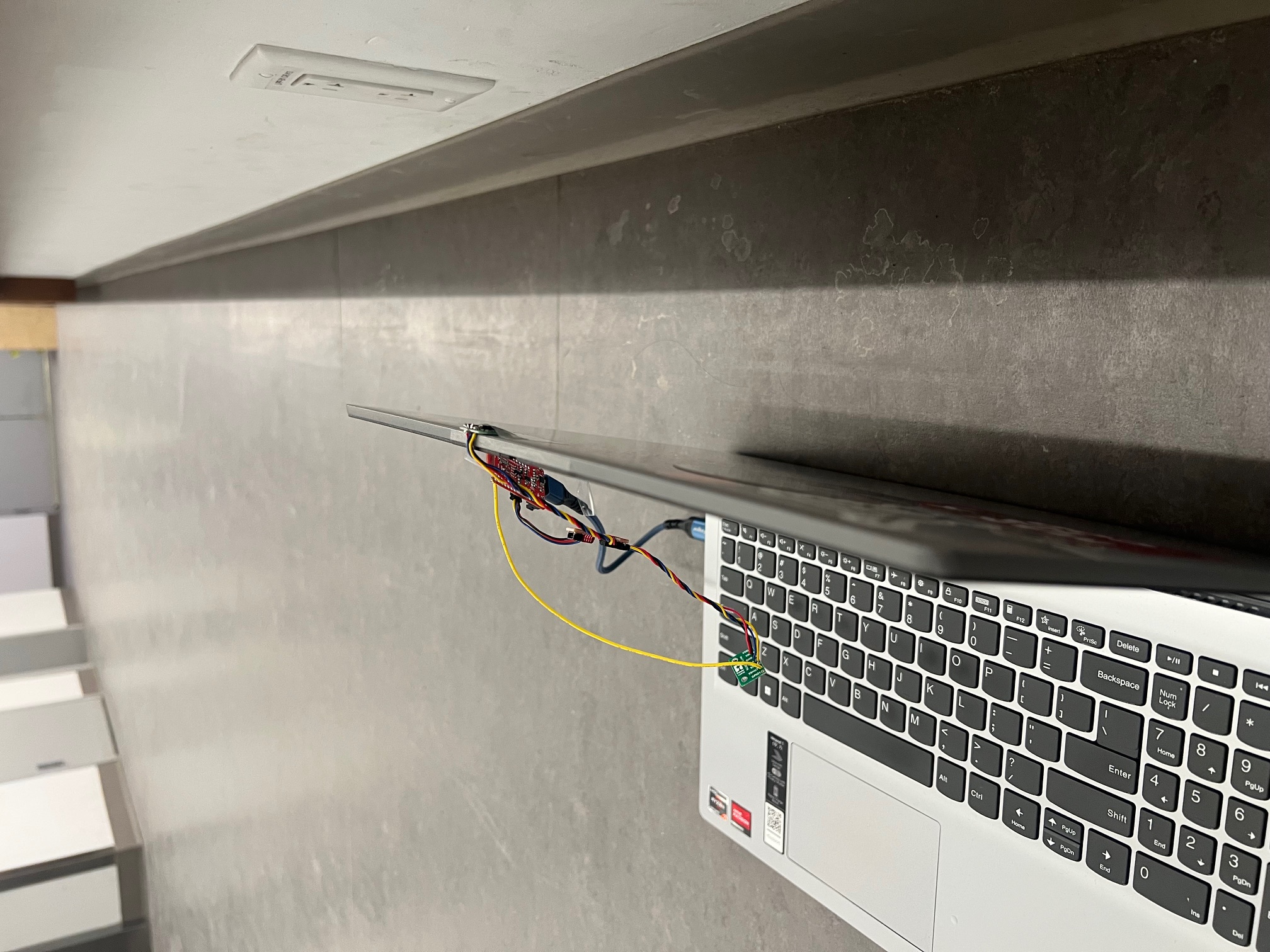
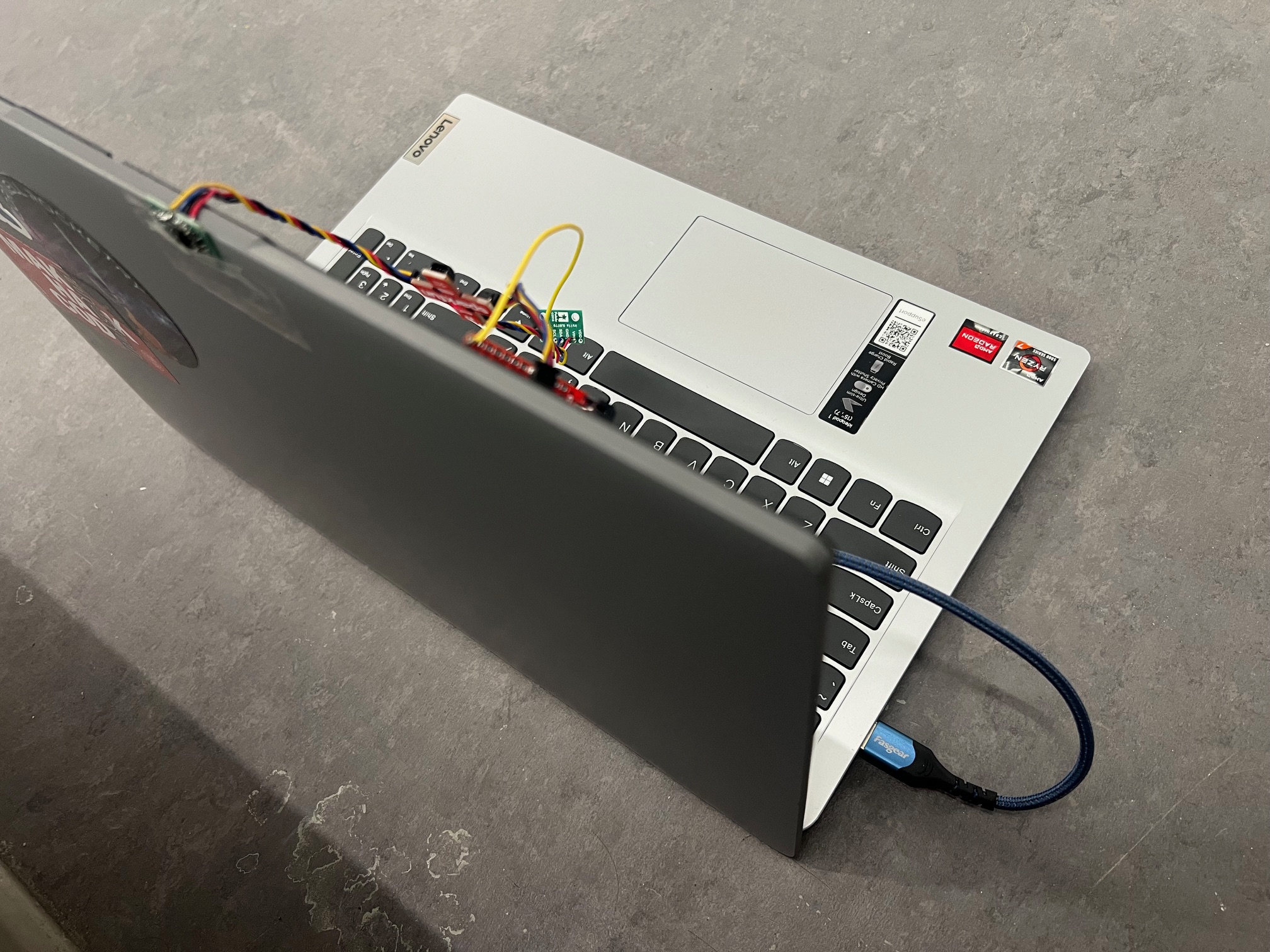
ToF Sensors' Position on the car
My plan for this lab was to position the two ToF sensors at the front and on the side of the car, hence I connected them next to each other relative to the QWIIC connector, as opposed to on the opposite sides of the connector. This seemed like to most optimal choice in my opinion, considering that the car will be able to detect the obstacles in front and to its side. Fo detecting the obstacles on the other side of the car or behind the car, we ought to rotate the car. The two ToF sensor correspond to the longer QWIIC connector cables, due to the fact that they require higher positionality dependence as opposed to the IMU.
Lab tasks
Testing the Time of Flight provided examples
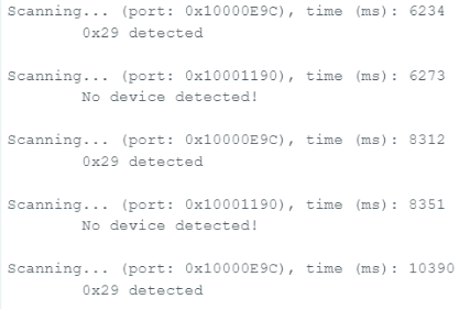
The XSHUT connection is not necessary for the initial ToF sensor testing. The first test was performed by using Example1_Wire_I2C under the Apollo3 library for scanning the I2C bus in order to verify the address of the sensor. The proposed output is as the following:
Discussion on I2C address
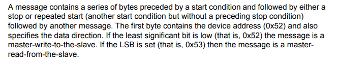
The indicated address is 0x29 which represents 0x52 bit shifted by 1, or 0x52 >> 1, thus negecting the last bit. The very last bit is supposed to represent the direction, thus 0 for a write and 1 for a read, hence we are paying attention to the first 7 bits, as can be confirmed from the ToF datasheet.
Chosen mode discussion
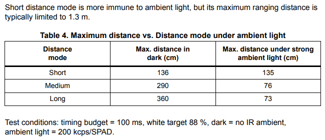
The mode that I chose was the Short Distance Mode, as according to the datasheet description, it has the sensor range of 1.3 meters and hence seems like a great fit for the proposed car. Furthermore, it has the best maximum distance under strong ambient light compared to other modes, adequate in this case.
Testing the chosen mode: Distance Mode SHort
The code for testing the proposed mode was adapted from SparkFun_VL53L1X_4m_Laser library's example named Example1_ReadDistance and incorporated in the ble_arduino.ino file.
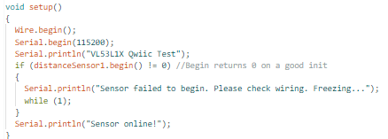
The setup for the sensor's distance detection looks like in the following images.
What is more, the distanceSensor1 was instantiated. Afterwards, I implemented a case called TIME_OF_FLIGHT as can be seen below, which enabled sending data over to Python for easier visualization of the data obtained.
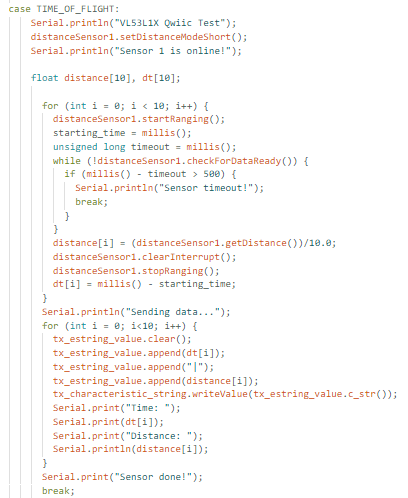
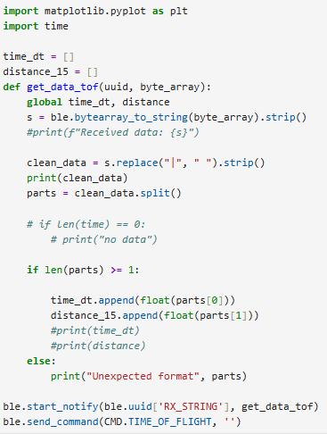
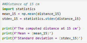
On the Python side, the code receiving the data for easier plotting will be as in the following images. Note, the second screenshot below represents the calculation of mean and standard deviation for the distance of 15 cm specificially. The calcultions were performed for distances for 15 cm to 150 cm, in increments of 15 cm.
After obtaining data for the proposed distance increments, we ought to compute ToF sensor range, accuracy, repeatability, and ranging time.
Sensor Range Discussion
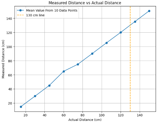
The proposed datasheet indicated that the short mode range of the ToF sensor is about 130 cm. In order to confirm the range myself, I tested the sensor behaviour at distances from 15 cm to 150 cm in increments of 15 cm. Hence, the graph below computed through the sent distance readings from Arduino displays the distance of ToF sensor to the wall. As shown in the "ToF Python code" figure, there were 10 means obtained for each distance measurements, and were plotted against the actual distances. The 130 cm line was indicated to display the proposed sensor range limit. There is a slight outlier at the 60 cm point mean measurement, which might be due to the sensor adapting to the new distance. The sensor range plot in the light and dark ambiance gives the same plot.
Accuracy Discussion
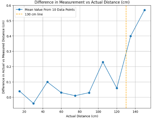
Similarly to the plot above, the accuracy plot is represented in the difference between the measured and the actual distances against the actual distances recorded from the ToF sensor to the wall. It can be observed that the accuracy is slightly worse as we increase the distance, which is to be expected considering the proposed sensor range in the datasheet. Once the 130 cm range line is passed, the accuracy of our ToF sensor visibly deteriorates. The sensor range plot in the light and dark ambiance gives the same plot.
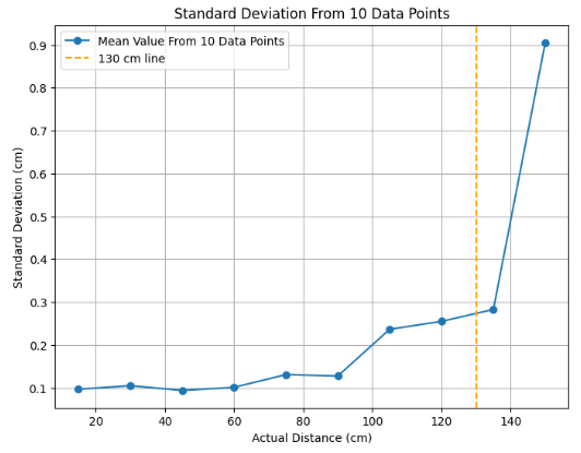
Repeatability Discussion
Repeatability is computed by calculating the standard deviation by utilizing statistics.stdev() on our recorded distance data, and afterwards computing it against the actual distance. Standard deviation is below 0.3 cm until the 130 cm range line indicated in orange, after which it significantly increases and reaches almost 1 cm at the distance of 150 cm, which is as expected considering the proposed graphs for accuracy and sensor range. The sensor range plot in the light and dark ambiance gives the same plot.
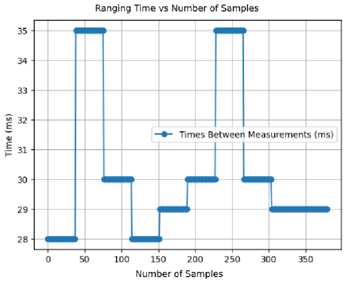
Ranging Time
As presented in the graph below, the ranging time of the samples taken at different distances was consistently under 35 ms with the aforementioned Arduino code. The loop time it takes to record the data samples ought to be optimized later in this lab report.
Two ToF Sensors Integrated
.jpg)
The initialization of 2 sensors requires for the second to be introduced as SFEVL53L1X distanceSensor2(Wire, XSHUT); and hence the code implemented in order to test that we wired the sensors propery and they can each detect accurate distances is shown below.
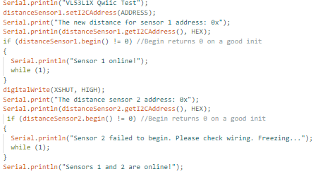
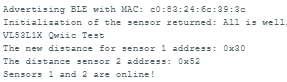
As can be seen in the figure above, the initialization displays that both of the sensors are correctly initialized with different non-conflicting addresses. The first ToF sensor now has to be written to a new address, that is 0x30, while the address of the newly initialized ToF sensor is 0x52.
Hence, we can run the code which allows for both of the sensor to output the distance data.
As can be concluded from the screenshot above, I varied the distances by simultaneously having both of my hands close to both ToF sensors, and then away from both ToF sensors, as can be reflected in sudden change of distances from very close to both sensors, to very distant from both sensors.
ToF Sensor Speed Optimization
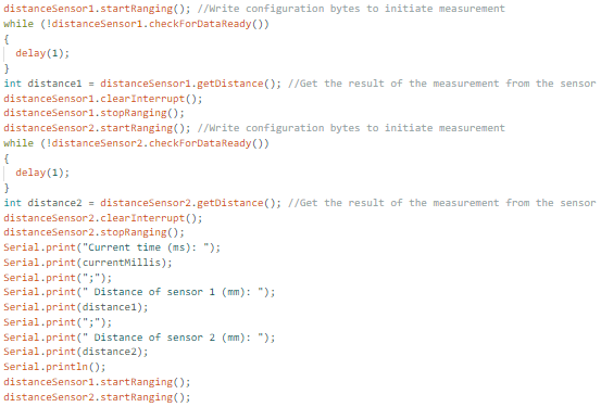
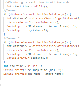
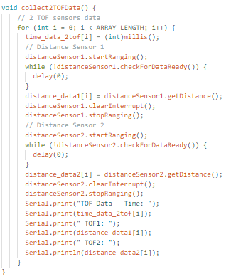
As proposed in the lab handout, the optimized execution of the code may be implemented by incorporating the distanceSensor.checkForDataReady() routine in order to determine when new data is available. This can be performed by implementing the following code in the loop() function.
Such optimization enabled data collection at a much faster rate, which ought to be detected in the following outputs. The first output showcases the loop at a slower rate, and the second screenshot showcases the optimized loop time output.
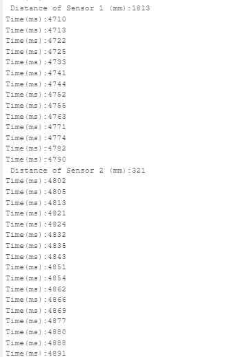
Hence, it can be concluded that the loop executes much faster with the implemented optimization, with loop time averaging to about 2-3 ms. The current limiting factor for this is not on our end, but purely the ability of the ToF sensors to acquire data.
ToF Sensors Data and IMU Data
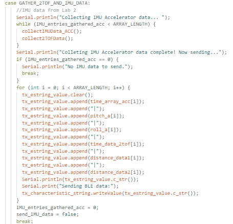
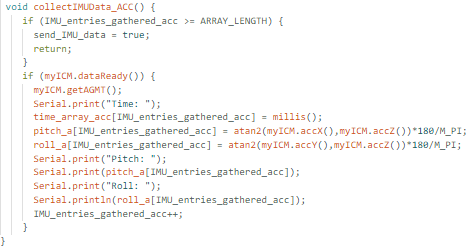
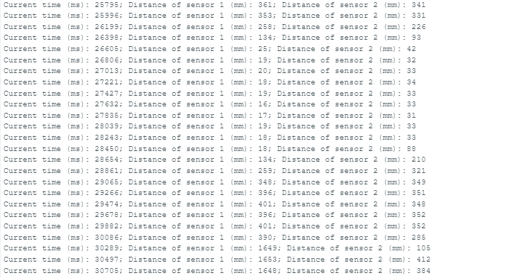
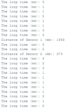
As can be seen from the provided code, the collectIMUData() code was adapted from Lab 2 code for the IMU. The case of GATHER_2ToF_AND_IMU_DATA was created in order to send the data as data packets to Arduino for easier plotting and analysis. In order to confirm that my 2 ToF sensor data was sending well, I printed them in the Serial Monitor and tested their distance recordings by varying the positions of my hands relative to the ToF sensors.
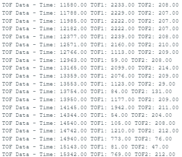
As can be seen in the Serial Monitor output above, it can be seen that distances recorded from ToF sensor 1 as opposed to ToF sensor 2 are opposite, and that is due to the fact that I varied my hand movement for one hand to be close to a ToF sensor while the other is away from the other ToF sensor, and vice versa. After determining that the ToF sensor distances are accurately measured, the data could be sent over Bluetooth, and thus plotted.
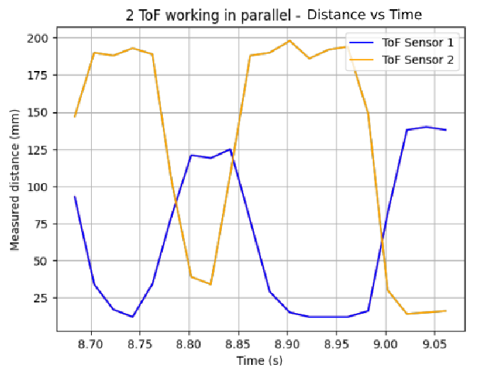
As can be seen from the aforementioned description of alternating the distances between the 2 ToF, when the first ToF sensor's distance is near the hand, the other's is far away, and vice versa, which matches the 2 ToF sensors' output at the Serial Monitor. On the other hand, the IMU data graph indicating the angle versus time may be plotted.
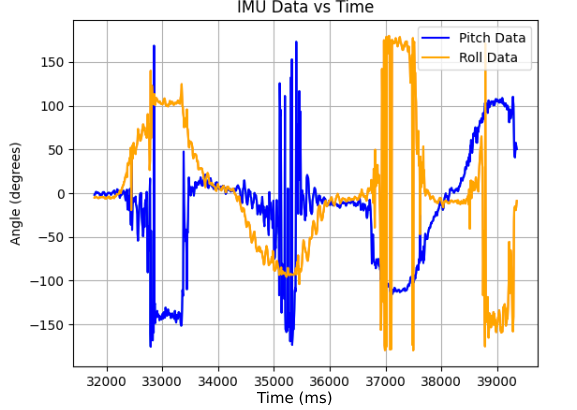
As can be inferred from the graph above, the pitch and roll data was varied so that the IMU is rotated in pitch direction first, and the in roll direction, and so on.
Additional tasks for 5000-level students
IR Sensor Discussion
This lab used an IR Time-of-Fligth sensor, however, more such IR sensors exist, some of which include amplitude-based IR sensors, and triangulation IR sensors. Amplitude-based IR sensors particularly work by sending IR pulses and then measuring the difference in amplitude of the received signal compared to the sent signal., while the radio determines distances of objects. Their pros are that they are relatively cheap, much cheaper than ToF IR sensors, as well as have straightforward calculations. However, they fundamentally work on short distances, as well as have high sensitivity to texture, colour, and light ambience - due to which time integration might be adjusted.
Another classification of IR sensors are the triangulation IR sensors, also known as angle-based IR sensors. These sensors operate by sending the IR pulse at an angle, and thus determining the angle at the receiving end, due to which the distance is determined. Some of the pros of these sensors are that they do not have sensitivity to colour or texture, and are of comparable price to the amplitude-based IR sesnors, as well as have a range up to 1 meter. However, the cons of this type of IR sensors is that they are bulky, and can be somewhat slow, as well as vary with the ambient lighting.
Lastly, ToF IR sensors have the highest range, much larger than the aforementioned two, are of small footprint, and do not have sensitivity to texture or colour. However, their cons are that they are much more expensive that the previous two types, as well as have more complex math behind them.
ToF Sensitivity to Colours and Textures Discussion
Considering that ToF sensors do not have sensitivity to colour or texture, the proposed may be determined with the sensors used in this lab. For this part of the lab, I varied two colours, red and blue, which I attached to the wall at a distance of 20 cm from the red and blue images. It can be determined from the videos below that colour did not have any affect on the sensitivity of the sensor, and the distance remained at 20 cm (the position of the ruler in the videos is maintained).
The second test performed was the test for texture, and the tested materials were a cardboard box and the wall. Similarly to the colour, it was determined that texture does not affect distance measured if the distance is set to a fixed distancewith a ruler. Hence, the ToF sensor is insensitive to texture as well. It can be observed that the distance from both textures to the ToF sensor is 20 cm.
Discussion
This lab provided me with new knowledge on how ToF sensors work, as well as made me become more cognizant about future steps of how I plan to attach the sensor to my robots and integrate them well.
*This lab page is inspired by TA Mikayla Lahr's Lab 3 page from Spring 2024.