LAB 5 - PID Control and Linear Interpolation
Introduction
The aim of this lab was to implement closed loop control and through the implementation of PID control. ToF sensors integrated in the third lab represented a crucial role in this lab as they ensured our robot stops at the target distance from the wall. PID control is consisted of proportional (P), integral (I), and derivative (D) control, where each of the terms evaluates the error between the desired position and the current position and adjusts the PWM signal of the motor accordingly.
Prelab 5
Sending and receiving data over Bluetooth
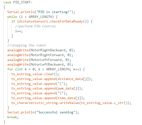
Considering that this lab is very dependent on value tuning for our implementation of the PID Control, as well as considering the fact that our robot is fundamtentally operating on the battery power throughout the lab, it was vital to establish a functional way of effective sending and receiving data. My solution to this consists of developing two cases in ble_arduino.ino, one named PID_START, which is responsible for collecting the data with the control loop implemneted, which allows collection while controling the car. The second case CHANGE_GAIN is responsible for transmitting the data through Bluetooth once the data collection is completed.
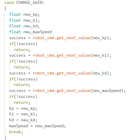
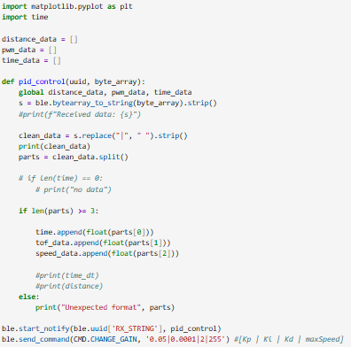
The proposed arrays sent over to Python side are thus separated and grouped into separate arrays for the purposes of plotting and analyzing the data. The Python script follows the same structure as the ones I wrote for notification handlers in previous labs. Furthermore, I call send_command in order to manipulate the values of Kp, Ki, Kd, and maxSpeed, as can be inferred from the comment in the image below.
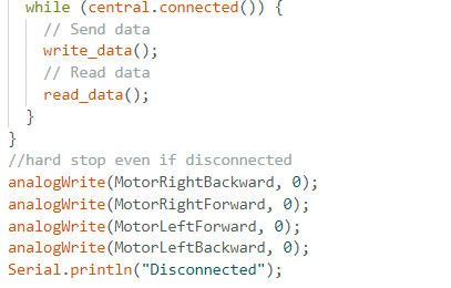
Another vital part of the prelab was ensuring that a hard stop is incorporated even in the cases of Bluetooth connection failing. I implemented this in the loop() function, as well as in the PID_START upon the completed data collection.
Lab 5 Tasks
PID Control Overview
Initially, I analyzed the formula for the motor input function u(t), which helped grasp the fundamentals of PID control. The PID controller, as aforementioned, is consisted of the proportional, integral, and derivative control portions, which form the motor input function u(t) as the following:
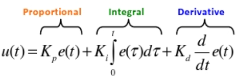
where e(t) is the error between the current position, measured by the ToF sensor, and the desired target position. Hence, P control seemed like a solid start point, considering that it has a fixed variable represented in the target distance. However, P controller is reflected in a considerable steady state error, due to the fact that it only responds to the present error, thus is not able to eradicate the persistent offset. Thus, implementing a PI controller is able to help this issue through providing the motors with a larger push until the error is diminished. The PID controller hence builds up on the established system through providing damping on the motor input due to fast changes in ToF sensor readings.
P Controller Implementation
With the provided analysis of my understanding of the formula, I started with the implementation of P controller. My implementation for the P controller can be found in the attached code below.
int t_0 = millis();
while ((i < ARRAY_LENGTH & millis()) - (t_0 < 5000)) {
    if(distanceSensor1.checkForDataReady())
    {
        distance1 =  distanceSensor1.getDistance();
        distanceSensor1.stopRanging();
        distanceSensor1.clearInterrupt();
        distanceSensor1.startRanging();
        i++;
    }
    // Start of Control Loop Calculations - P Control
    distance_data1[i] = distance1;
    current_distance = distance1;
    old_error = error1;
    error1 = target_dist - current_dist;
    dt = millis() - prev_time;
    prev_time = millis();
    p_term = Kp * error1;
    i_term = 0;
    d_term = 0;
    pwm = p_term + i_term + d_term
Furthermore, the forward and backward movement control is implemented similarly to Lab 4, by using analogWrite() statements for when different values of PWM. The code for wheels movemment is attached in the PID Control Implementation code below (*considering that I tested my code on Kelvin's car as mentioned in References below), I had to change my naming convention for wheel's pin outputs to adapt to his hardware.
When testing the P controller, I varied different values of Kp, while keeping my Ki and Kd equal to 0. Furthermore, I varied the values of maxSpeed as well to observe the behaviour of the controller. Depending on the speed, the ranges of my Kp values varied from 0.03 to 0.07 when testing, and these values experimentally proved to have the most accurate results of detecting the distance target, but also moving in a straight line without noticeable jittering. Furthermore, with the optimal value of Kp being 0.05, an error of 100 mm would only yield about 5% of speed, which is a sensible achievement for a large distance up to 4 meters of long range mode.
The video representing the P controller ought to be found below. Through experimentation and tuning, I concluded that the Kp value that contributes to the achievable distance of 1 ft from the target is Kp = 0.028.
PI Controller Implementation
In order to introduce the integrator term, I subtract previous time instance from millis() in order to obtain dt, which I multiply with the calculated error between the target distance and the current distance. Hence, keeping track of the previous loop time allows me to calculate dt and sum the error over time. The more we loop, the more impactful integrator portion of the equation becomes, thus the more we divide by dt, the larger the error.
The video representing the PI controller ought to be found below. Tuning the values, I chose Kp = 0.025, Ki = 0.001, and maxSpeed = 100, while keeping Kd = 0.
...//while loop
    }
    // Start of Control Loop Calculations - PI Control
    distance_data1[i] = distance1;
    current_distance = distance1;
    old_error = error1;
    error1 = target_dist - current_dist;
    dt = millis() - prev_time;
    prev_time = millis();
    error_sum = error_sum + (error1*dt/1000);
    p_term = Kp * error1;
    i_term = Ki * error_sum;
    d_term = 0;
    pwm = p_term + i_term + d_term;
    ...//pwm values control
Upon tuning the values, I observed that in the instances where PI controller overshoots and hits the wall, it is able to recover the robot to the desired distance, which effectively makes sense with the integrator error equation. Such example can be found in the video below.
PID Controller Implementation
Finally, the PID controller ought to be implemented by accounting for the derivative d_term in our code. Below is the full implementation of PID controller. The derivative term is obtained by determining the change in error between the previous step and the current step and thus dividing by dt. I chose to implement PID controller instead of PI, as I wanted to create a more robust mechanism, and introduce the damping term into the equation in order to reduce oscillations and overshooting, as well as to achieve a more stable system response through counteracting changes in proposed error.
case START_PID:
{
    int i = 0;
    int k = 0;
    float target_dist = 304;
    int distance1 = 0;
    float current_dist;
    float error1;
    float pwm;
    float error_sum;
    float p_term, i_term, d_term;
    float old_error;
    float dt_extrapolate;
    float distance_before_last;
    float distance_last;
    float time_before_last;
    float time_last;
    float slope;
    float time_current;
    float b, m, x;

    distanceSensor1.startRanging();
    Serial.println("PID is starting!");
    int t_0 = millis();
    // This is used to calculate dt
    int prev_time = t_0;
    while ((i < ARRAY_LENGTH) && (millis() - t_0 < 10000)) {
        if (distanceSensor1.checkForDataReady()) {
            distance1 = distanceSensor1.getDistance();
            distanceSensor1.stopRanging();
            distanceSensor1.clearInterrupt();
            distanceSensor1.startRanging();
            i++
        }
        // Start of Control Loop Calculations - PID
        distance_data[i] = distance1;
        current_dist = distance1;
        old_error = error1;
        dt = millis() - prev_time;
        error1 = target_dist - current_dist;
        prev_time = millis();
        time_data[i] = prev_time;
        error_sum = error_sum + (error1 * dt / 1000);
        p_term = Kp * error1;
        i_term = Ki * error_sum;
        //d_term = 0;
        d_term = Kd * (error1 - old_error)/dt;
        pwm = p_term + i_term + d_term;
        Serial.println(pwm);

        // Movement Saturation and Control
        if (pwm > maxSpeed) pwm = maxSpeed;
        if (pwm < -maxSpeed) pwm = -maxSpeed;
        pwm_data[i] = pwm;
        if (pwm > 0) { //forward movement
            analogWrite(MotorRightBackward, 0);
            analogWrite(MotorRightForward, pwm + 5);
            analogWrite(MotorLeftForward, pwm * 2.0 + 12);
            analogWrite(MotorLeftBackward, 0);
        } else if (pwm < 0) { //backward movement
            analogWrite(MotorRightBackward, abs(pwm) + 5);
            analogWrite(MotorRightForward, 0);
            analogWrite(MotorLeftForward, 0);
            analogWrite(MotorLeftBackward, abs(pwm) * 2.0 + 12);
        } else { //stopping the robot
            analogWrite(MotorRightBackward, 0);
            analogWrite(MotorRightForward, 0);
            analogWrite(MotorLeftForward, 0);
            analogWrite(MotorLeftBackward, 0);
        }
    } //implementing hard stop
    analogWrite(MotorRightBackward, 0);
    analogWrite(MotorRightForward, 0);
    analogWrite(MotorLeftForward, 0);
    analogWrite(MotorLeftBackward, 0);

    for (int k = 0; k < ARRAY_LENGTH; k++) {
        tx_estring_value.clear();
        tx_estring_value.append(distance_data[k]);
        tx_estring_value.append("|");
        tx_estring_value.append(pwm_data[k]);
        tx_estring_value.append("|");
        tx_estring_value.append(time_data[k]);
        tx_characteristic_string.writeValue(tx_estring_value.c_str());
    }
    Serial.println("Successful sending");
    break;
} // case end
Here are the instances of testing the implemented PID controller. It can be observed that Ki value is set to the smallest value due to its augmenting nature, while Kd term is set to be the highest value in magnitude compared to Kp or Ki due to the fact that it can help with the provided damping on the robot so that it does not overshoot.
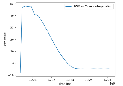
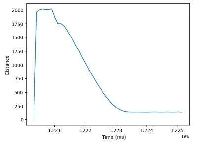
The data collected from the proposed videos was generated to obtain the motor input versus time as well as ToF versus time graphs. Such graphs can be observed below.
Linear Extrapolation
The following task of the lab was to implement linear extrapolation, which can be comprehended as a prediction mechanism in case our ToF sensor's values are not available for collection, that is, when distanceSensor1.checkForDataReady() is not available. Hence, in case of obtaining 2 ToF values, the data points in-between measurements are used to determine the location of the robot. This was performed through adding an else if () statement to my PID control code, integrated into the while loop for whenever distanceSensor1 data is not available. This way, the collected data arrays are supposed to have more frequent and accurate data collection due to the fact we are able to frequently loop in the else statement and speed up the controller execution.
    while ((i < ARRAY_LENGTH) && (millis() - t_0 < 10000)) {
        if (distanceSensor1.checkForDataReady()) {
            distance1 = distanceSensor1.getDistance();
            distanceSensor1.stopRanging();
            distanceSensor1.clearInterrupt();
            distanceSensor1.startRanging();
        } else if (i > 1) {
            time_current = millis();
            distance_last = distance_data[i - 1];
            distance_before_last = distance_data[i - 2];
            time_last = time_data[i - 1];
            time_before_last = time_data[i - 2];
            slope = (distance_last - distance_before_last) / (time_last - time_before_last);
            b = distance_last;
            m = slope;
            x = time_current - time_last;
            distance1 = b + m * x;
        }
        // Start of Control Loop Calculations - PID
Implementing the proposed code, in the START_PID case and integrating it before executed PID control resulted in producing the following video below (thanks to TA Cameron for filming the video!).
Speed and Sampling Time discussion
When it comes to the range of ToF sensors, in previous lab 3 we have determined that even though the ToF sensor's datasheet describes the range of the long mode to be about 1.3 meters, the control signal is saturated regardless, even if the distance is above 1.3 m. Hence, the acceleration towards the wall even in the range up to 2 meters or so. On the other hand, with precision, short range mode would probably be more precise, but only a small increment, especially with a large derivative portion of the control.
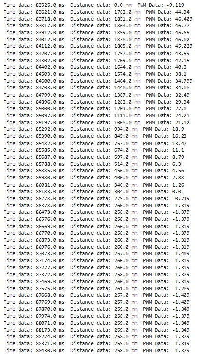
When it comes to the sampling time, upon performing PID control without the linear extrapolation, I noticed that the sampling time initially was calculated to be in the range of 100 ms per measurement, as can be seen in the image below. This was the original calculation of the ToF reading when the sensor was ready for the data. However, when the linear extrapolation was implemented, this allowed for the estimation to be performed while the sensor was not ready for data collection, and thus the while() loop executed at a much faster rate. Hence, the loop speed was measured to range to about 20-30 ms per time reading. Furthermore, this matches how fast the sensor runs, which corresponds to about 50 Hz for the long range mode.
What is more, for the purposes of updating the ToF sensor frequency, I also considered the statements for timing budget and intermeasurement period of the sensor, as described in the sensor library. I placed the below code in the loop() function, thus, setting the timing budget and intermeasurement period can benefit the ToF sampling time.
Additional ECE 5160 Tasks
Wind-up
Lastly, wind-up protection for the integrator term of the PID Controller can be introduced, as it represents the vital feature for robust PID Control. I implemented the wind-up protection through clamping the integrator term in order to prevent any further error from accumulating for a longer period beyond the set limit. Otherwise, the integrator term can accumulate the excessive error, which can lead the robot to overshoot in positionality, thus making it harder and longer for the robot to stabilize. Hence, wind-up protection may be implemented as the following:
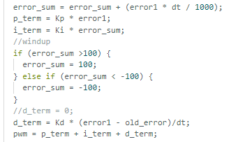
By tuning and manipulating the values of the limit, I decided that the limit of +/- 100 seemed fitting. Furthermore, I tested the wind-up implementation by varying Ki values on the Python side in order to evaluate the respose of the system. I found that even with larger Ki values of 0.001 or 0.0001 magnitude, the car could reach stability in front of the target distance, which normally was not the case with such large integrator term input. The wind-up performance on the system can be inferred in the video below.
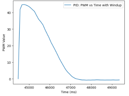
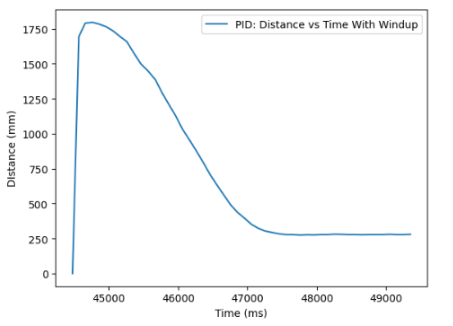
What is more, with the linear extrapolation implemented, as well as the wind-up protection, the graphs generated below represent the final results of ToF versus Time as well as with the linear extrapolation and wind-up protection implemented on the PID Controller.
Discussion
This lab was crucial in gaining a better understanding of closed loop control and experimenting with PI and PID Control implementation. Furthermore, it enabled me great exprience in debugging, tuning values, and evaluating the best solution for the robot with its open-endedness.
Acknowledgements and References
*This lab page is inspired by Nila Narayan's and Stephan Wagner's Page (2024). I worked with Kelvin Resch, and Paul Judge on this lab. I shared ideas with Becky Le and Sabian Grier as well. The videos were filmed on Kelvin Resch's car as discussed with the Professor, due to my car's hardware breaking upon the lab deadline.