LAB 6 - ORIENTATION CONTROL
Introduction
The aim of this lab was to build up on the demonstrated PID control with lateral movement from lab 5, by developing the mechanism to control the orientation angle of our motor. More particularly, yaw measurements of the IMU were utilized in order to implement a PID controller that is able to point the car towards a particular target yaw angle, as well as maintain the orientation.
Prelab 6
Sending and receiving data over Bluetooth
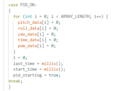
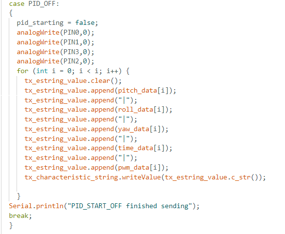
Considering that this lab is very dependent on value tuning for our implementation of the orientation angle and PID parameters, as well as considering the fact that our robot is fundamtentally operating on the battery power throughout the lab, it was vital to establish a functional way of effective sending and receiving data. My solution to this is influenced by my Prelab 5 code, where I developed the case PID_ON, which is responsible for collecting the different pieces of data for, which will be relevant for testing and controlling the orientation of our car. Similarly, there is a flag pid_starting incorporated in the code attached below, and the boolean is thus set to true once the data arrays are cleared . Similarly, there is another case PID_OFF, which ends the control loop and thus implements a hard stop on the robot's wheels, after which it sends the populated arrays from Arduino over Bluetooth.
The code for both of the cases can be seen below:
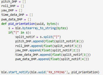
The proposed arrays sent over to Python side are thus grouped into separate arrays for the purposes of plotting and analyzing the data. The Python script follows the same structure as the ones I wrote for notification handlers in Lab 5.
Lab 6 Tasks
Digital Motion Processing (DMP)
The fundamental purpose of Digital Motion Processing (DMP) is to incorporate different sensor readings obtained through using the IMU data, which ultimately and ideally ought to decrease noise levels from the accelerometer, as well as the drift from the gyroscope, which was experienced in Lab 2. Digital Motion Processing enables low-power calibration of the accelerometer, gyroscope, and compass, while maintaining optimal performance of the sensor data. DMP is integrated into the Artemis Board, and through the quick uncommenting of line 29 in the ICM_20948_C.h header file, as suggested by the Lab 6 website documentation, we may test its functionality through the Arduino example sketch: Examples > SparkFun 9DoF IMU Breakout > Arduino > Example7_DMP_Quat6_EulerAngles. The test proved the functionality, by displaying the expected behaviour of pitch, roll, and yaw angles in real-time.
Furthermore, I was able to recall the gyroscope readings and the experienced drift in Lab 2, and thought about how I ought to mitigate such drift throughout this lab. While collecting IMU data, I determined that smaller inaccuracies build up the drift, resulting in a larger measured angle as the error accumulates over time. In order to minimize the drift, the gyroscope bias ought to be subtracted from the gyroscope readings. Therefore, utilizing DMP can correct the drift due to it incorporating gyroscope, accelerometer, and magnetometer measurements.
I started analyzing the DMP behaviour by testing the Arduino example sketch: Examples > ICM 20948 > Arduino > Example6_DMP_Quat9_Orientation, which helped me determine how to read orientation data in quarternion form. The sketch helped me further realise how the gyroscope readings are combined with the accelerometer data, contributing to the DMP correcting its initial exhibited drift. By utilizing the tutorial code on DMP, as well as the code provided on the attached Wikipedia page in the tutorial, I was able to adapt my setup() function to account for the following:
bool success = true; // In order to confirm that the DMP configuration was successful
// Initialize the DMP. initializeDMP is a weak function. You can overwrite it if you want to e.g. to change the sample rate
success &= (myICM.initializeDMP() == ICM_20948_Stat_Ok);
// Enable the DMP Game Rotation Vector sensor
success &= (myICM.enableDMPSensor(INV_ICM20948_SENSOR_GAME_ROTATION_VECTOR) == ICM_20948_Stat_Ok);
success &= (myICM.setDMPODRrate(DMP_ODR_Reg_Quat6, 4) == ICM_20948_Stat_Ok); // Set to the maximum

// Enable the FIFO
success &= (myICM.enableFIFO() == ICM_20948_Stat_Ok);

// Enable the DMP
success &= (myICM.enableDMP() == ICM_20948_Stat_Ok);

// Reset DMP
success &= (myICM.resetDMP() == ICM_20948_Stat_Ok);

// Reset FIFO
success &= (myICM.resetFIFO() == ICM_20948_Stat_Ok);

// Check success
if (success)
{
    Serial.println("DMP success!");
}
else
{
    Serial.println(F("Enable DMP failed!"));
    Serial.println(F("Please check that you have uncommented line 29 (#define ICM_20948_USE_DMP) in ICM_20948_C.h..."));
    while (1); // Do nothing more
}
Furthermore, by following the documentation, I learned how to take DMP orientation measurements as quarternions and convert them into an Euler angle for rotation about the z-axis, which is represented in yaw angle. This is performed by incorporating the following code snippet into my main code for obtaining the pitch, roll, and yaw data.
icm_20948_DMP_data_t data;
myICM.readDMPdataFromFIFO(&data);
if((myICM.status == ICM_20948_Stat_Ok) || (myICM.status == ICM_20948_Stat_FIFOMoreDataAvail))
{
    if ((data.header & DMP_header_bitmap_Quat6) > 0)
    {

    double q1 = ((double)data.Quat6.Data.Q1) / 1073741824.0; // Convert to double. Divide by 2^30
    double q2 = ((double)data.Quat6.Data.Q2) / 1073741824.0; // Convert to double. Divide by 2^30
    double q3 = ((double)data.Quat6.Data.Q3) / 1073741824.0; // Convert to double. Divide by 2^30
    double q0 = sqrt(1.0 - ((q1 * q1) + (q2 * q2) + (q3 * q3)));

    double qw = q0;
    double qx = q2;
    double qy = q1;
    double qz = -q3;

    // roll (x-axis rotation)
    double t0 = +2.0 * (qw * qx + qy * qz);
    double t1 = +1.0 - 2.0 * (qx * qx + qy * qy);
    double roll = atan2(t0, t1) * 180.0 / PI;
    roll_data[i] = roll;

    // pitch (y-axis rotation)
    double t2 = +2.0 * (qw * qy - qx * qz);
    t2 = t2 > 1.0 ? 1.0 : t2;
    t2 = t2 < -1.0 ? -1.0 : t2;
    double pitch = asin(t2) * 180.0 / PI;
    pitch_data[i] = pitch;

    // yaw (z-axis rotation)
    double t3 = +2.0 * (qw * qz + qx * qy);
    double t4 = +1.0 - 2.0 * (qy * qy + qz * qz);
    double yaw = atan2(t3, t4) * 180.0 / PI;
    yaw_data[i] = yaw;
    time_data[i] = millis();
    i++;
As can be seen, I am storing my pitch, roll, and yaw values into arrays, which I ought to transmit to Python for easier analysis. An important thing to note, is that the aforementioned Example6_DMP_Quat9_Orientation helped me investigate the correct the orientation of my robot depending on the outputted yaw angles. Hence, through experimenting, I determined that when my PWM value is negative, and there is a negative difference between my target and my current yaw value, the motion of my car ought to be clockwise. This was incredibly useful when configuring the motion for my car to orient towards the desired angle.
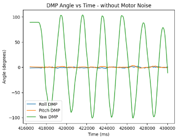
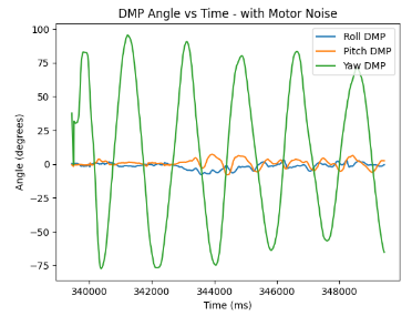
For testing purposes, I plotted the the transmitted pitch, roll, and yaw data to investigate the initial behaviour by only rotating yaw in the cases of stationary robot, and robot with motors rotating.
P Controller Implementation
Similarly to how I implemented P Controller in Lab 5, I incorporated the following code after performing the DMP quarternion orientation measurements and obtaining pitch, roll and yaw arrays, and created a PID_DMP_TURN case for sending my angle arrays, as well as my PWM and time data arrays. The code placed in the case can be found below:
//the following variables are set globally
int i = 0;
unsigned long last_time = millis();
double target_yaw = -30;
double current_yaw = 0;
float dt = 0;
float error_pid;
float pwm;
float error_sum = 0.0;
float p_term = 0.0;
float i_term = 0.0;
float d_term = 0.0;
float old_error;
//end of global variable definitions

case PID_DMP_TURN: {

//DMP quarternion code snippet attached above which stores roll_data[i], pitch_data[i], yaw_data[i], and time_data[i] values
...
// yaw (z-axis rotation)
double t3 = +2.0 * (qw * qz + qx * qy);
double t4 = +1.0 - 2.0 * (qy * qy + qz * qz);
double yaw = atan2(t3, t4) * 180.0 / PI;
yaw_data[i] = yaw;
...
// end of DMP code snippet

dt = (millis()-last_time);
last_time = millis();
current_yaw = yaw;
old_error = error1;
error1 = current_yaw-target_yaw;
//P Control
error_sum = error_sum + error1*dt;
p_term = Kp * error1;
i_term = 0;
d_term = 0;
pwm = p_term + i_term + d_term;
p_term_data[i] = p_term;

if(pwm > 0)
{
    if(pwm > maxSpeed)
    pwm = maxSpeed;
}
else if(pwm < 0)
{
    if(pwm < -maxSpeed)
    pwm = -maxSpeed;
}
pwm_data[i] = pwm;
    if(pwm < -80) { // needs to be clockwise motion because yaw difference is negative
        analogWrite(PIN0,abs(pwm)); //right backward
        analogWrite(PIN1,0); // right foward
        analogWrite(PIN3,abs(pwm)); //left forward
        analogWrite(PIN2,0); // left backward
    }
    else if(pwm > 80) // 80 was determined to be the minimum spinning PWM in Lab 4
        {
        analogWrite(PIN0,0);
        analogWrite(PIN1,abs(pwm));
        analogWrite(PIN3,0);
        analogWrite(PIN2,abs(pwm));
    else{
        analogWrite(PIN0,0);
        analogWrite(PIN1,0);
        analogWrite(PIN3,0);
        analogWrite(PIN2,0);
    }
}
if (myICM.status != ICM_20948_Stat_FIFOMoreDataAvail) // if more data is available then we should read it right away - and not delay
{
delay(10);
}

for (int j = 0; j < i; j++) {
    tx_estring_value.clear();
    tx_estring_value.append(pitch_data[j]);
    tx_estring_value.append("|");
    tx_estring_value.append(roll_data[j]);
    tx_estring_value.append("|");
    tx_estring_value.append(yaw_data[j]);
    tx_estring_value.append("|");
    tx_estring_value.append(time_data[j]);
    tx_estring_value.append("|");
    tx_estring_value.append(pwm_data[j]);
    tx_estring_value.append("|");
    tx_estring_value.append(p_term_data[j]);
    tx_characteristic_string.writeValue(tx_estring_value.c_str());
  }
Serial.println("PID turning data sent!");
break;
}
As can be seen from the P Controller code provided above, the code largely adapts the Lab 5 code for P Controller. The commented code for DMP quarternion orientation calculations is displayed in the code snippet attached in the Digital Motion Processing (DMP) subsection of this webpage. As can be seen from the code, arrays storing PWM data, time data, roll data, pitch data, yaw data, and P term data are sent over to Python for analysis. The notable difference in the P Controller form the previous lab is the fact that we set our current yaw to be the yaw computed in the DMP quarternion snippet, after which the error for P term is computed by taking the difference between the current yaw and the target yaw we would like to achieve. Furthermore, as can be inferred from the global definitions, the target yaw in this case was set to -30 degrees.
Another update from Lab 5 code for P Controller was the spinning of the wheels depending on the PWM value. It was determined that with the negative PWM value, as aforementioned, we ought to move clockwise as determined via experimentation, due to the negative difference between the current yaw value and the target yaw value. Since I am only focusing on the P term for now, I term and D term may be set to 0 on the Arduino side, as well as when running the CHANGE_GAIN case on the Python side, which, similarly to Lab 5, looks as the following attached snippet. CHANGE_GAIN enables manipulating Kp, Ki, Kd, and the speed of the rotating wheels, or maxSpeed value.

Initially, when testing only the P Controller, I was able to set my Kp value to be Kp = 3, while keeping Ki and Kd terms equal to 0. Below is the video of my tuned P Controller. In initial stages of testing, I had the car plugged into my Artemis while adjusting its movement to reach the desired angle, due to the fact that I wanted to print out my angles while the robot was moving in order to determine that the target yaw was reached. This can be seen in the video as well. The target yaw is set to -30 degrees from the starting point in the video.
Furthermore, I wanted to experiment with performing the P Controller kick in order to observe the behaviour of my implemented system. Below are the videos trying to achieve the same target yaw of -30 degrees.
As can be inferred from the videos, the first P Controller kick example shows that the controller still overshoots a bit, after which it readjusts to orient itself towards the desired angle. The second video represents a similar behaviour, where overshooting is followed up by undershooting until the robot balances itself to the desired angle value.
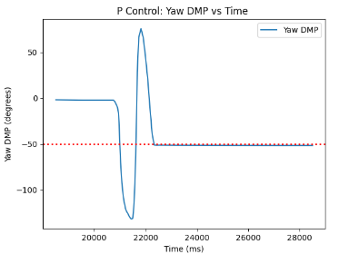
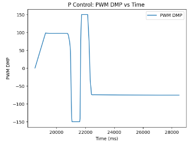
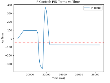
Through experimentation I was able to plot graphs from the collected data arrays, which can be found below. The graphs represent my experimentation with -50 as my target yaw for the plots.
PI COntroller Implementation
Afterwards, I incorporated the integral term into my code. While the proportional term has, as demonstrated, got me fairly close to the desired target angle, the system is still quite unstable. Furthermore, in the case of a distinctly large or small Kp value, we could experience overshooting or undershooting to the setpoint. Therefore, we ought to incorporate the integral term in order to account for this, thus achieving a higher stability of the system and getting closer to the setpoint. As can be inferred from the attached code snippet below, the only addition to our PI Controller as opposed to the P Controller is that the integral term is consisted of adding up the error based on the difference in time which is thus multiplied by the desired Ki value. Hence, every such summation is added to the new error_sum value, as can be seen below.
//...DMP code snippet
dt = (millis()-last_time);
last_time = millis();
current_yaw = yaw;
old_error = error1;
error1 = current_yaw-target_yaw;
//PI Control
error_sum = error_sum + error1*dt;
i_term = Ki * error_sum;
pwm = p_term + i_term + d_term;
p_term_data[i] = p_term;
i_term_data[i] = i_term;
//... PWM code, the same as in P Controller code snippet above
The final Kp and Ki terms that I have tuned to be the most optimal for my robot's PI Controller were Kp = 2.8, Ki = 0.00001, and Kd = 0, since the derivative term is not incorporated yet.
Below are the videos representing the initial tuning of the PI Controller, the PI Controller kick, as well as the tuned PI Controller. The desired yaw value for all of the instances is -30 degrees relative to the starting position of the car, where the wheels are lined up with the edge of the tiles to represent starting position of the robot on the 2D space.
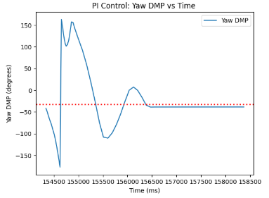
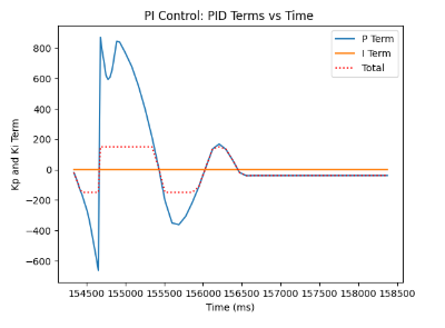
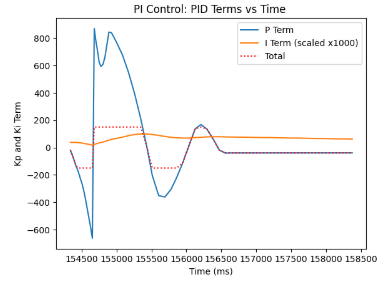
Through experimentation, I was able to obtain the following plots representing the PI Controller. The fourth attached graph was rescaled for I term for easier analysis of the term's behaviour. As can be inferred from the graphs below, the target yaw is -30 degrees, and the car initially overshot, only to undershoot until it stabilized into the desired angle value. Furthermore, we can see how the I term impacted the behaviour of our plots, the static error accumulates, which is why the trend goes up for I term when overshooting, and after the desired yaw value is achieved, the I term slowly deteriorates.

PID Controller Implementation
Lastly, the derivative D term was incorporated into the code. The code is updated from the previous PI Controller to account for D term.
//...DMP code snippet
dt = (millis()-last_time);
last_time = millis();
current_yaw = yaw;
old_error = error1;
error1 = current_yaw-target_yaw;
//PID Control
error_sum = error_sum + error1*dt;
p_term = Kp * error1;
i_term = Ki * error_sum;
d_term = Kd * (error1 - old_error)/dt;
pwm = p_term + i_term + d_term;
p_term_data[i] = p_term;
i_term_data[i] = i_term;
d_term_data[i] = d_term;
//... PWM code, the same as in PI Controller code snippet above
//
...
///
for (int j = 0; j < i; j++) {
    // if(time_data[j] == 0)
    // break;

    tx_estring_value.clear();
    tx_estring_value.append(pitch_data[j]);
    tx_estring_value.append("|");
    tx_estring_value.append(roll_data[j]);
    tx_estring_value.append("|");
    tx_estring_value.append(yaw_data[j]);
    tx_estring_value.append("|");
    tx_estring_value.append(time_data[j]);
    tx_estring_value.append("|");
    tx_estring_value.append(pwm_data[j]);
    tx_estring_value.append("|");
    tx_estring_value.append(p_term_data[j]);
    tx_estring_value.append("|");
    tx_estring_value.append(i_term_data[j]);
    tx_estring_value.append("|");
    tx_estring_value.append(d_term_data[j]);
    tx_characteristic_string.writeValue(tx_estring_value.c_str());

  }
Normally, it is not efficient to take the derivative of yaw integrated over time from gyroscope's angular velocity data, however, due to the fact that discrete angle readings are provided by DMP, derivative ought to be performed.
Performing a derivative of an integrated signal may be problematic in the context of utilizing DMP. Considering that integration accumulates errors, differentation may amplify the noise, thus if derivative of yaw from the DMP ought to result in small fluctuations or noise amplifications, which may lead to instability of PID Controller. Hence, derivative might not reflect meaningful physical changes except the dominant drift/noise, which ought to be the reason why filtering is applied. However, considering that with good tuning my system was resilient to noise and was able to perform well, filtering was not applied to the derivative term.
Another significant point of discussion with PID orientation control is suddent change of the setpoint, which ought to create instantaneous error accumulating into a spike in the control output. Ultimately, this may cause more aggressive and sudden movements, which are not desirable in systems such as PID orientation where robot stability is crucial. Therefore, in order for the error to be minimized, we ought to implement the wind-up of the integral term, which will be covered in the subsection below.
Below are the videos representing the tuning of the PID Controller, the PID Controller kicks. The desired yaw value for all of the instances is -30 degrees relative to the starting position of the car, where the wheels are lined up with the edge of the tiles to represent starting position of the robot on the 2D space.
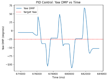
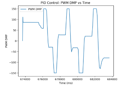
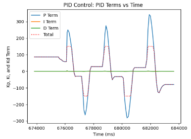
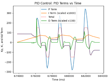
The final Kp and Ki terms that I have tuned to be the most optimal for my robot's PI Controller were Kp = 2.2, Ki = 0.00001, and Kd = 2. As can be seen, the system is more resilient to overshooting, and is able to more accurately predict future errors by measuring how fast the error is changing, which effectively is the property of the derivative term. Ultimately, tuning the values led me to obtaining the following graphs, which represent the PID Controller.
Speed and Sampling Time discussion
Considering that we are not dealing with a Time-of-Flight sensor like in Lab 5, we expect the control loop to speed up by a lot. In order to compute the loop frequency and the data frequency, I performed the following code in Python based on the received time data array.
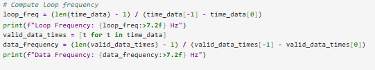
It was observed that the loop frequency is about 52 Hz, while the data drequency is about 49.3 Hz. Hence the DMP is capable of keeping up with the control loop, in a much better manner than with our Lab 5 computer loop frequency.
Additional ECE 5160 Tasks
Wind-up
Lastly, as aformenetioned in PID Controller Implementation, the wind-up protection for the integrator term can be introduced, as it represents the crucial feature for robust PID Control. I implemented the wind-up protection through clamping the integrator term, similarly to Lab 5, in order to prevent any further error from accumulating for a longer period beyond the set limit. Otherwise, our integrator term can accumulate the excessive error, which can lead the robot to overshoot in positionality, thus making it harder and longer for the robot to stabilize. Hence, wind-up protection may be implemented as the following:
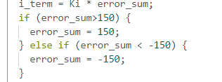
By tuning and manipulating the values of the limit, I decided that the limit of +/- 150 seemed fitting. Furthermore, I tested the wind-up implementation by varying Ki values on the Python side in order to evaluate the respose of the system. I found that even with larger Ki values of 0.001 or 0.0001 magnitude, the car could reach stability in front of the target yaw angle, which was generally not the case with such large integrator term input. The wind-up performance on the system can be inferred in the video below.
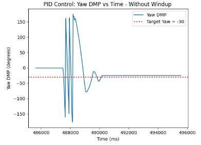
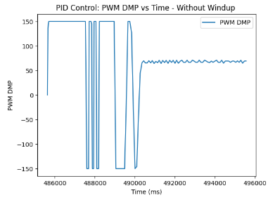
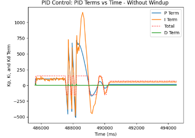
Here is my PID without wind-up. As can be seen, the orientation control tends to spin in circles until reaching the target yaw angle of -30 relative to the starting position. This is due to the fact that the yaw error is large for an extended period, which results in the growing integral term. Hence, there is an increasing control output, which can cause overcorrection and thus overshooting of the target, as represented in the PID without Windup video below.
Thus, integral wind-up can be implemented as in the code above, which limits error values larger than 150 to the value of 150, and error values smaller than -150 to the value of -150. The improved PID Control with wind-up can be seen in the video below.
What is more, we can plot the graphs with and without the implemented wind-up protection. As can be seen, the graphs with wind-up protection display several instances of picking up the robot and placing it at random positions on the ground for it to recalibrate and determine the same exact target yaw angle of -30 degrees.
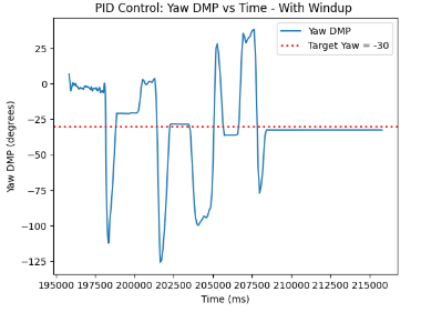
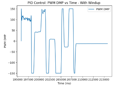
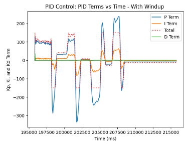
On the other hand, with the graphs of PID Control without wind-up protection, we can detect consecutive spinning until the value stabilizes and reaches the targeted yaw angle.
Discussion
This lab was crucial in gaining a better understanding the benefits of Digital Motion Processing, as well as gaining experience with Orientation Control. Furthermore, it enabled me great exprience in debugging, tuning values, and evaluating the best solution for the robot with its open-endedness.
Acknowledgements and References
*I worked with Paul Judge, and Aravind Ramaswami on this lab.