LAB 7

Introduction

The aim of this lab was to gain a more profound understanding of the Kalman Filter through implementing it in Python, as well as implementing it on our robot. The addition of the Kalman FIlter onto the collected Lab 5 data results in a faster executional behaviour compared to Lab 5. Kalman Filter is specifically designed to handle state estimations in the presence of noisy sensor measurements and disturbances. Furthermore, Kalman Filtering is extremely useful as it produces a predictive model for state estimations even in the cases of missing or delayed sensor measurements, as well as continuously updating the estimate with the newly measured data, which makes it effective in dynamically changing environments. However, unlike linear extrapolation performed in Lab 5, which uses the current rate of change to estimate future states and assumes a linear model without accounting for uncertainties, Kalman Filter considers process noise and measurement (sensor) noise, incorporating a state-space model predicting system behaviour over time.

Prelab 7

Throughout Lab 5, the timing budget proposed was 20 ms for the loop speed, which results in the ToF distance sensing at the frequency of 50 Hz. This was the result of linear extrapolation on the PID Controller, which was able to perform predictions of the intermediate readings based on the previous two data points. In this lab, however, the predictions and updates of the future robot movement was implemented in a more accurate way accounting for noise-resistant state estimation.

Lab 7 Tasks

Estimating Drag and Momentum

In order to obtain a deeper understanding of how the Kalman Filter works, I consulted Lecture 13 slides in order to plan out my first calculations. From the lecture, we revisited that by Newton's second law of motion we have:

Furthermore, we know that the linear force on the robot in terms of drag d can be descrived as the following:

where u is the motor input u. Setting the two formulas equal and dividing by mass m, we can describe the system dynamics in the following formula.

From here, we are able to obtain our state-space equations. We can do so by taking our system modeling equation \( \dot{x} = Ax + Bu \) , where \(A\) represents the current state matrix, \(B\) represents the control input matrix, \(u\) represents the control input to the system, and \( \dot{x}\) represents the range of change of the state variables over time. The state of the system can be represented as a vector:

Furthermore, the expression of \(\ddot{x}\) can be represented in the system equation form:

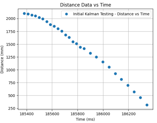
Finally, I drove my car to the wall in order to save arrays containing my ToF distance values, time values, and had the constant PWM input of 170, which is 66.7% as my step response u(t). Hence, I determined the following graphs displaying my Distance versus Time measurement.

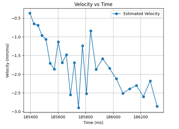
Furthermore, the Speed versus Time graph can thus be obtained by taking the difference of the obtained distance measurements and dividing it by the change in time. The graph ought to look as the following:

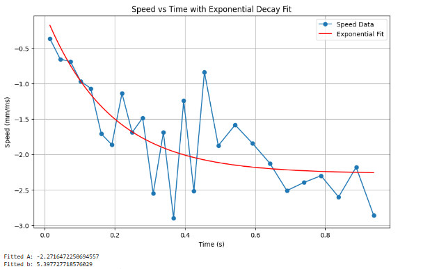
From there, we ought to observe the exponential trend of the Speed versus Time graph. For further determining the drag d and the mass m coefficients, we ought to implement the following formula.

\[ d = \frac{u_{ss}}{\dot{x}_{ss}} \]

\[ m = \frac{-d \cdot t_{0.9}}{\ln(1 - d \cdot \dot{x}_{ss})} = \frac{-d \cdot t_{0.9}}{\ln(1 - 0.9)} \]

where \(u_{ss}\) is the steady state input, \(\dot{x}_{ss}\) is the steady state speed, and \(t_{0.9}\) represents the 90% rise time. However, since the noise in the graphs presented are quite noisy, it became difficult to determine where to exactly measure the 90% rise time and the speed at 90% rise time. Thus, an exponential curve was fitted to the speed versus time data.

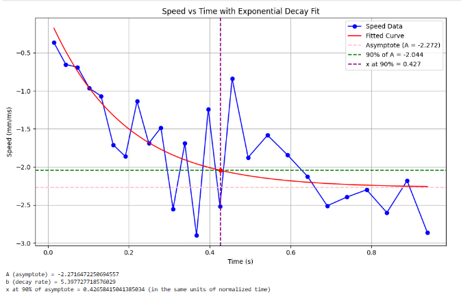
The obtained parameters will become very useful in the remaining portion of our Python implementation shortly. Analyzing our Distance versus Time graph, we ought to identify a linear region corresponding to the achieved steady state speed near the end of the wall run.

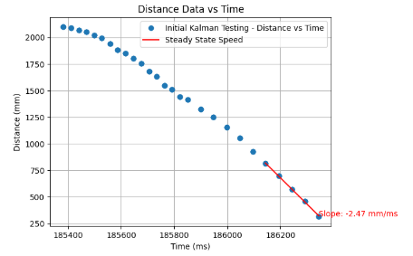
Analyzing the presented graphs indicating Speed versus Time with the Exponential Decay Fit, as well as the calculated steady state speed indicated on the graph above and the aforementioned formulas, we have obtained vital information in determining the drag d as well as the mass m. From the analysis of the two graphs above, it can be inferred that the steady state speed \(\dot{x}_{ss}\) is 2.47 m/s, the 90% rise time is calculated on the exponential fit graph to be 0.427 s, and the speed at 90% rise time is 2.044 m/s. Hence, thedrag and mass of the system can be computed as the following:

\[ d = \frac{u_{ss}}{\dot{x}_{ss}} = \frac{1}{2.47 m/s} = 0.405 kg/s \]

\[ m = \frac{-d \cdot t_{0.9}}{\ln(1 - d \cdot \dot{x}_{ss})} = \frac{-d \cdot t_{0.9}}{\ln(1 - 0.9)} = \frac{-0.405 kg/s \cdot 0.427 s}{\ln(0.1)} = 0.075 kg \]

Initialize the Kalman Filter

Afterwards, we ought to discretize A and B matrices in order to simulate the Kalman Filter in Python. From the previously presented formulas, we learned that \( \dot{x} = Ax + Bu \), where we can represent matrices A and B as:

The proposed matrices can be discretized using the Python code:

import numpy as np

# Define the continuous-time A and B matrices
A = np.array([[0, 1],
                [0, -5.3977]])
B = np.array([[0],
                [113.3]])

# Sampling time
dt = 0.02  # 20 ms

# Dimension of the state space
n = 2

# Discretization
Ad = np.eye(n) + dt * A
Bd = dt * B

print("Discretized A (Ad):")
print(Ad)
print("\nDiscretized B (Bd):")
print(Bd)
print(dt)

The sampling time dt indicated in the code above was determined through determining the loop frequency, and calculating 1/{loop frequency}, which in my case gave the value of 0.02. Hence, the discretized matrices were calculated as the following:

Furthermore, it is important to note that we ought to incorporate the C matrix as well, representing the states measured. The lecture slides proposed a negative coefficient, however, I turned that into a positive coefficient instead in order to represent the positive distance data.

This can be reflected in the following Python code implementation:

time_data = np.array(time_data[start_point:end_point]) - time[start_point]
tof_data = tof_data[start_point:end_point]
uss = 1

C = np.array([[1, 0]]) # Initialized C matrix
x = np.array([[-tof_data[0]], [0]]) # tof from collected data

The ultimate step of the Python initialization of the Kalman Filter was to make estimations for both process and measurement noise. They are defined based on the sampling time dt and the sensor variance dx, and can be expressed by the following expressions. The first two represent the process noise, while sigma 3 represents the sensor noise.

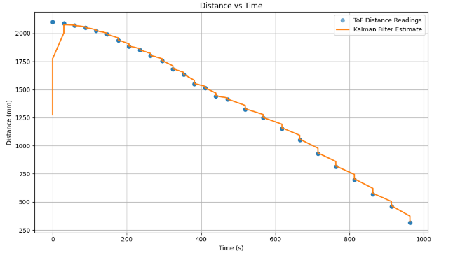
As previously mentioned, the sampling time for the position as well as velocity is determined by the ToF sampling period of 20 ms. For the sensor noise, I examined the datasheet of the ToF sensors in order to match the ranging error at long-distance proposed by the manufacturer, as in the following diagram for long range distance:

Hence, we can define convariances and diagonal convariance matrices \( \sum_u\) and \( \sum_z\).

The process noise \( \sigma_1\) and \( \sigma_2\) were set to 70 each, as we would like to have higher reliance on the measurements. The code implementing the noise can be found below:

# Process noise
sigma_1 = 70
sigma_2 = 70

# Sensor noise
sigma_3 = 20

sigma_u = np.array([[sigma_1**2, 0], [0, sigma_2**2]]) 
sigma_z = np.array([[sigma_3**2]]) 

Implementation in Python

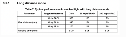
After we have initialized all the required matrices and variables, we ought to implement a Kalman Filter function in order to process the data. I based my function on the code provided in lecture slides. Furthermore, I made an upade in my function only if the sensor readings are valid:

def kalman_filter(mu, sigma, u, y, update = True):
    mu_p = Ad.dot(mu) + Bd.dot(u) 
    sigma_p = Ad.dot(sigma.dot(Ad.transpose())) + sigma_u
    if update == False:
        return mu_p, sigma_p
    sigma_m = C.dot(sigma_p.dot(C.transpose())) + sigma_z
    kkf_gain = sigma_p.dot(C.transpose().dot(np.linalg.inv(sigma_m)))

    y_m = y - C.dot(mu_p)
    mu = mu_p + kkf_gain.dot(y_m)
    sigma = (np.eye(2) - kkf_gain.dot(C)).dot(sigma_p)

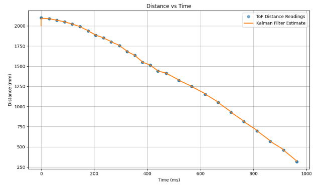
    return mu, sigma

Afterwards, I was able to plot the data which proves that the Kalman filter is able to interpolate in-between the measured ToF data points. The following graphs will show the importance of covariance matrices. Particularly, with the increase in sensor noise covariance, the Kalman Filter ultimately puts much higher trust in the model, which causes it to estimate states which differ from the measurements from the ToF sensor. That would be great in the application where the dynamic model is very accurate, but the sensors performing the measurements were noisy. However, considering that our ToF sensors are decently accurate, the best tuned Kalman Filter is the one shown in the first graph below, where the sensor covariance was the lowest (\( \sigma_3\)), while model covariances (\( \sigma_1\) and \( \sigma_2\)) were much larger than sensor covariance.

Kalman Filter Implementation on the Robot

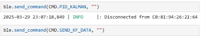
The Kalman Filter implementation on the robot ended up more challenging, as it required some thinking about how to perform the prediction step through code. I started off by having a separate case called SEND_KF_DATA, which will send the collected arrays for ToF distance, as well as the computed Kalman Filter distance, and the time. The code is similar to the one writeen in the previous labs and can be found below.

case SEND_KF_DATA: 
    for (int k = 0; k < ARRAY_LENGTH; k++) {
        if (time_data[k] == 0) break;
        else {
        tx_estring_value.clear();
        tx_estring_value.append(distance_data1[k]);
        tx_estring_value.append("|");
        tx_estring_value.append(pwm_data[k]);
        tx_estring_value.append("|");
        tx_estring_value.append(time_data[k]);
        tx_estring_value.append("|");
        tx_estring_value.append(kf_distance_array[k]);
        tx_estring_value.append("|");
        tx_estring_value.append(kf_time[k]);
        tx_characteristic_string.writeValue(tx_estring_value.c_str());
        Serial.println(tx_characteristic_string);
        }
    }
    Serial.println("Finished sending Kalman Filter data!");
    break;
}
                            

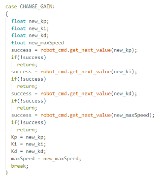
In order to change the set Kp, Ki, Kd, and maxSpeed values (the speed of the car ranging 0-255), I utilized the function written in Lab 5 CHANGE_GAIN. The code included from Lab 5 can be found below:

On the Python side, I instantiated a notification handler similar how I coded it in previous labs. I

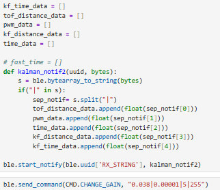
After simulating the Kalman Filter in Python, I instantiated the required matrices used in the Python implementation.

float d = 0.405;
float t_r = 0.42659;
float m = (-d*t_r)/log(.1);

float sigma_1 = 70;
float sigma_2 = 70;
float sigma_3 = 20;

Matrix<2,2> A = {0, 1,
        0, -1*(d/m)}; 
Matrix<2,1> B = {1, 15*(1/m)}; 
Matrix<1,2> C = {1,0}; 

float Delta_T = 0.02; # 20 ms
Matrix<2,2> I = {1, 0,
                    0, 1};
Matrix<2,2> Ad;
// Ad  = I + Delta_T * A ;
Matrix<2,1> Bd;
// Bd = Delta_T * B;
Matrix<1,2> Cd;
// Cd = C;

Matrix<2,2> sigma_u = {sigma_1*sigma_1, 0,
                        0, sigma_2*sigma_2};
Matrix<1> sigma_z = {sigma_3*sigma_3};
Matrix<2,1> mu_p;
Matrix<2,2> sigma_p;
Matrix<1> sigma_m;
Matrix<2,1> kkf_gain;
Matrix<1> y_m;
Matrix<1> y;
Matrix<2,1> mu = {1,0}; //{set_distance, 0}
Matrix<2,2> sigma = {400, 0, 
                0, 100};

Matrix<1> u = {1};

Afterwards, Kalman Filter was implemented into my Lab 5 PID controller lab code. The full code displaying the update and prediction steps for the Kalman Filter is shown below

case PID_KALMAN: 
{
    //...PID variable instantiation from Lab 5
    float kf_distance;

    Ad  = I + Delta_T * A ;
    Bd = Delta_T * B;
    Cd = C;

    distanceSensor1.startRanging();  //Write configuration bytes to initiate measurement
    Serial.println("Staring Kalman Filter with PID!");
    int t_0 = millis();
    int prev_time = t_0;
    while (!distanceSensor1.checkForDataReady())
    {
        delay(1);
    }
    distance1 =  distanceSensor1.getDistance();
    distanceSensor1.clearInterrupt();
    mu = {(float) distance1, 0.0};
    while ((i < ARRAY_LENGTH && j < ARRAY_LENGTH2) && millis() - t_0 < 5000) {
    time_data[i] = millis();
    if (distanceSensor1.checkForDataReady()) { //ToF sensor data available
        dt = millis() - prev_time;
        prev_time = millis();
        distance1 = distanceSensor1.getDistance();  //Get the result of the measurement from the sensor
        distanceSensor1.clearInterrupt();
        distance_data1[i] = distance1;
        i++;
        y = (float) distance1; //y(0,0) = (float) distance1;
        mu_p = Ad*mu + Bd*u;
        sigma_p = Ad*sigma*~Ad + sigma_u;
        sigma_m = Cd*sigma_p*~Cd + sigma_z;
        kkf_gain = sigma_p*~Cd*Inverse(sigma_m);
        y_m = y-Cd*mu_p;
        mu = mu_p + kkf_gain * y_m;
        sigma = I - kkf_gain*Cd*sigma_p;
        kf_distance = mu(0,0);
        kf_distance = (float) kf_distance;
        if (j < ARRAY_LENGTH2) { 
        kf_distance_array[j] = kf_distance;
        kf_time[j] = millis();
        j++;
        }
        // Start of Control Loop Calculations
        current_dist = distance1;
        distance1 = mu(0,0);
        old_error = error1;
        error1 = current_dist - target_dist; 
        //PID Control from Lab 5
        error_sum = error_sum + (error1 * dt / 1000);
        p_term = Kp * error1;
        i_term = Ki * error_sum;
        d_term = Kd * (error1 - old_error) / dt;
        pwm = p_term + i_term + d_term;
    }
    else{ // ToF sensor data not available, make predictions with Kalman Filter
        mu_p = Ad*mu + Bd*u;
        sigma_p = Ad*sigma*~Ad + sigma_u;
        kf_distance = mu_p(0,0);
        kf_distance = (float) kf_distance;
        mu = mu_p;
        sigma = sigma_p;
        if (j < ARRAY_LENGTH2) { 
        kf_distance_array[j] = kf_distance;
        kf_time[j] = millis();
        j++;
        }
        dt = millis() - prev_time;
        prev_time = millis();
        current_dist = kf_distance;
        old_error = error1;
        error1 = current_dist - target_dist; 
        //PID Control from Lab 5
        error_sum = error_sum + (error1 * dt / 1000);
        p_term = Kp * error1;
        i_term = Ki * error_sum;
        d_term = Kd * (error1 - old_error) / dt;
        pwm = p_term + i_term + d_term;
    }
    // Update motors the same way as in Lab 5
    break;
}

The provided code for PID_KALMAN works in such a way where I incorporate an update step incorporating valid ToF readings with the PID loop code from Lab 5. I started the update step by taking my code from Lab 5, incorporating the matrices and variable updates per each iteration as per the provided code in lecture slides, and ensured that my PID update step is functional. Afterwards, I introduced a separate counter variable j in order to loop through the Kalman filter distances which are dependent on the computed mu value. Afterwards, the computed KF distances are appended to the Kalman Filter distances array, while ToF recorded distances were appended to the separate ToF distances array, similarly to how they were appended in Lab 5.

However, there is a point to note. Firstly, I found it quite challenging, but rewarding to finally see the Kalman Filter implemented on the robot. Some of the issues I have had during the runs is my ToF sensor data updating very slowly, which I was able to confirm through sampling time code in python provided in Lab 5 and 6. I was able to solve the issue through incorporating

for my sensor, which fixed the issue.

Afterward, I was ready to work on the predicton step, which would enable Kalman Filter functionality and prediction for when ToF sensor data is not available. Hence, with the attached final iteration of the code above, if the update step runs of the Kalman Filter runs, then the distance measurement is used as per the ToF reading (labeled as //ToF sensor data available in the code). Otherwise, if the prediction step runs, then we ought to take the most recent value of mu in the PID controller.

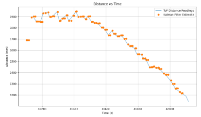
Furthermore, I had slight issues where the filter is predicting the distances between ToF readings, due to the fact that the predicted values did not follow the trend of the data towards the next update value, this can be reflected in the first trial with my prediction step implemented below, where my prediction step was more similar to the previous update step on the graphs attached below:

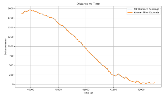
In order to fix this, I consulted with TA Mikayla who shared that she delt with the same issue in her implementation last year, and advised me to multiply my B matrix with a certain positive integer constant, in order to have the noise in the trend of the data follow the slope better. I settled for multiplying matrix B by the value of 10 and achieved the following results:

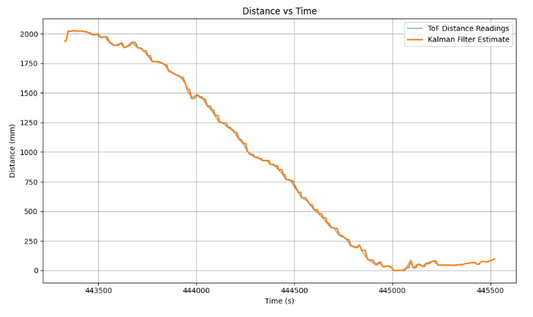
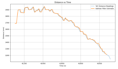
Furthemore, I was able to obtain the following graphs after tuning:

The video representation can be shown below. All of the videos were filmed with the tuned values of Kp = 0.35, Ki = 0.00001, and Kd = 5. The speeds were varied to be 220-255 for the purposes of these videos.

Discussion

This lab was crucial in gaining a better understanding the benefits of the Kalman Filter. Furthermore, it enabled me great exprience in debugging, tuning values, and evaluating the best solution for the robot with its open-endedness.

DEBUGGING AND COMMENTS on faced issues

One of the issues which slowed my process down was not adapting my Delta_T value needed for the discrediced Ad and Bd matrices in my robot implementation Kalman Filter code to the actual sampling time of my ToF sensor data. Once I ran the code for sampling time from Lab 6, as well as determined the sampling time of ToF sensors is about 20 ms as per Serial print statements, I was able to obtain much less noisy Kalman Filter data, and more accurate predictions once the ToF sensor data was not available.

Acknowledgements and References

*I worked with Sabian Grier on this lab. My lab page is inspired by Mikayla Lahr's (2024) and Stephan Wagner's Lab 7 page (2024). Super special thanks to TA Mikayla for her great advice on Robot implementation of Kalman Filter, as well as TA Cheney and TA Cameron for their insights on understanding Kalman Filter better. Furthermore, since my motor drivers overheated and broke in the earlier stages of testing my Kalman filter, Kelvin lent me his car for initial testing. The code is entirely mine.