LAB 9 - Mapping
Introduction
The aim of this lab is to familiarize ourselves with the technique of mapping by utilizing the ToF sensor readings, and doing so by mapping the static room that was set up in the class lab space. The map set up by the instructors will further be used in localization and navigation labs later on.
The primary goal of the lab was to successfully collect ToF readings and map the obstacles and walls of the room that was set up in the lab, based on four different marked locations within the composed static room. There were various possible approaches to this lab, however, I chose to solve it through utilizing knowledge obtained in Lab 6 on Digital Motion Processing (DMP), which enabled me to obtain consistent ToF readings through keeping track of my measured and expected yaw values, through proposing consistent angular increments.
Control and Obtaining ToF Readings
As aforementioned, I opted for approaching the lab through implementing closed-loop control using DMP as per obtained Lab 6 knowledge, which ought to help me obtain low-noise angle measurements for the yaw. Upon defining my global variables, I obtain the initial yaw value through setting a while loop which reads the quarternion from the IMU and successfully converts it inot a yaw value, similarly to how we performed the measurement in Lab 6. The code for this can be found below:
icm_20948_DMP_data_t data;
distanceSensor0.startRanging();

// Obtain the initial yaw
while (true) {
    myICM.readDMPdataFromFIFO(&data);
    if ((myICM.status == ICM_20948_Stat_Ok || myICM.status == ICM_20948_Stat_FIFOMoreDataAvail) &&
        (data.header & DMP_header_bitmap_Quat6)) {
    double q1 = ((double)data.Quat6.Data.Q1) / 1073741824.0;
    double q2 = ((double)data.Quat6.Data.Q2) / 1073741824.0;
    double q3 = ((double)data.Quat6.Data.Q3) / 1073741824.0;
    double q0 = sqrt(1.0 - ((q1 * q1) + (q2 * q2) + (q3 * q3)));
    double qw = q0, qx = q2, qy = q1, qz = -q3;
    double t3 = 2.0 * (qw * qz + qx * qy);
    double t4 = 1.0 - 2.0 * (qy * qy + qz * qz);
    initial_yaw = atan2(t3, t4) * 180.0 / PI;
    break;
    }
    for (int step = 0; step < steps; step++) {
        target_yaw = initial_yaw + step * yaw_step;
        if (target_yaw > 180) target_yaw -= 360;
        if (target_yaw < -180) target_yaw += 360;
    //...Perform PID Turn Loop//
}
Furthermore, I initiate distanceSensor0.startRanging(); function on the sensor before starting PID control on the robot in order to start the sensor's timing budget. Afterwards, I perform the calculations of my next target yaw at every angle increment of 10 degrees. The for loop was set to have the total number of steps to be 37, in order to compute the full circle in increments of 10. The further update of target yaw normalizes the values to be within the range of [-180 degrees, 180 degrees] through decrementing 360 degrees if target yaw is greater than 180, and incrementing 360 degrees for the cases of target yaw being smaller than -180 degrees, in order to achieve consistency. Furthermore, this is also performed in order to maintain PID control, as we would not want to perform unnecessary turns of our robot due to a miscalculation in the error (since the target yaw is subtracted from current yaw angle, and hence if target yaw were to be negative and close to -180, it would induce a large positive angle which would initiate the excessive turning, while in reality the turn could be of a much smaller angle if normalized - for instance, error = current_yaw - target_yaw = -178 - (-178) = 356, which should have yielded the turn of 4 degrees instead).
Afterwards, PID Loop Control is established in order to reach the successive target yaw values, as can be seen in the code portion attached below. The PID control is performed based on the equations proposed in Lab 5, and error is computed upon every step increment of 10 degrees. With setting the error less than 2 degrees check, we ensure that we avoid infinite loops, annd accept a small yet precise tolerance to noise, checking the preciseness of the target angle constantly. What is more, the set timeout for the sensor is 3 seconds, after which the robot is programmed to perform a stop, as can be seen in the full lab code section attached below.
for (int step = 0; step < steps; step++) {
    target_yaw = initial_yaw + step * yaw_step;
    if (target_yaw > 180) target_yaw -= 360;
    if (target_yaw < -180) target_yaw += 360;

    bool targetReached = false;
    unsigned long turnStartTime = millis();

    // PID Turn Loop
    while (!targetReached && millis() - turnStartTime < 2000) {
        myICM.readDMPdataFromFIFO(&data);
        if ((myICM.status == ICM_20948_Stat_Ok || myICM.status == ICM_20948_Stat_FIFOMoreDataAvail) &&
            (data.header & DMP_header_bitmap_Quat6)) {

        double q1 = ((double)data.Quat6.Data.Q1) / 1073741824.0;
        double q2 = ((double)data.Quat6.Data.Q2) / 1073741824.0;
        double q3 = ((double)data.Quat6.Data.Q3) / 1073741824.0;
        double q0 = sqrt(1.0 - ((q1 * q1) + (q2 * q2) + (q3 * q3)));
        double qw = q0, qx = q2, qy = q1, qz = -q3;
        double t3 = 2.0 * (qw * qz + qx * qy);
        double t4 = 1.0 - 2.0 * (qy * qy + qz * qz);
        current_yaw = atan2(t3, t4) * 180.0 / PI;

        dt = (millis() - last_time) / 1000.0;
        last_time = millis();

        error = current_yaw - target_yaw;
        if (error > 180) error -= 360;
        if (error < -180) error += 360;

        error_sum += error * dt;
        if (error_sum > 150) error_sum = 150;
        if (error_sum < -150) error_sum = -150;

        p_term = Kp * error;
        i_term = Ki * error_sum;
        d_term = Kd * (error - prev_error) / dt;
        pwm = p_term + i_term + d_term;

        prev_error = error;

        if (abs(error) < 2.0) {
            targetReached = true;
            break;
        }
//...Perform motor rotation code//
Lastly, the Tof distance reading is collected upon performing a one second delay which enables accurate sensor reading. Furthermore, the sensor is reset for the next ToF reading through performing distanceSensor0.clearInterrupt();, as well as distanceSensor0.stopRanging(); and then starting the sensor again through distanceSensor0.startRanging();. The accumulated values for the particular step increment in the total of 37 steps are appended to their respective arrays, and sent over through Bluetooth to Python for plotting and easier analysis. The arrays I sent over for plotting were the expected yaw measurements, recorded yaw measurements, times they were recorded, as well as the ToF distances at that particular angle and timestamp readings.
    //Get distance
    int distance_tof = 0;
    if (distanceSensor0.checkForDataReady()) {
        distance_tof = distanceSensor0.getDistance();
        distanceSensor0.clearInterrupt();
        distanceSensor0.stopRanging();
        distanceSensor0.startRanging();
        Serial.println(distance_tof);
    }

    // Save data to arrays
    expected_yaw_data[step] = step * 10;
    actual_yaw_data[step] = current_yaw;
    timestamps[step] = millis();
    tof_data[step] = distance_tof;
}

//Send collected data arrays
for (int j = 0; j < steps; j++) {
    tx_estring_value.clear();
    tx_estring_value.append(expected_yaw_data[j]);
    tx_estring_value.append("|");
    tx_estring_value.append(actual_yaw_data[j]);
    tx_estring_value.append("|");
    tx_estring_value.append(timestamps[j]);
    tx_estring_value.append("|");
    tx_estring_value.append(tof_data[j]);
    tx_characteristic_string.writeValue(tx_estring_value.c_str());
}
For reference, a full code used for the lab is inclulded below. It ought to be clarified that I used a calibration constant of 1.1 which I multiplied with the pin outputs representing the left set of wheels, as was determined in lab 4.
Full lab code shown here for reference
case PID_TURN_FULL:
{
    const int steps = 37;
    const float yaw_step = 10.0;
    double initial_yaw = 0;
    double target_yaw, current_yaw;
    float error = 0, prev_error = 0, error_sum = 0;
    float dt = 0;
    float pwm = 0, p_term, i_term, d_term;
    unsigned long last_time = millis();

    // Arrays for logging set as global variables
    // double actual_yaw_data[steps];
    // double expected_yaw_data[steps];
    // unsigned long timestamps[steps];
    // int tof_data[steps];

    icm_20948_DMP_data_t data;
    distanceSensor0.startRanging();

    // Obtain the initial yaw
    while (true) {
    myICM.readDMPdataFromFIFO(&data);
    if ((myICM.status == ICM_20948_Stat_Ok || myICM.status == ICM_20948_Stat_FIFOMoreDataAvail) &&
        (data.header & DMP_header_bitmap_Quat6)) {
        double q1 = ((double)data.Quat6.Data.Q1) / 1073741824.0;
        double q2 = ((double)data.Quat6.Data.Q2) / 1073741824.0;
        double q3 = ((double)data.Quat6.Data.Q3) / 1073741824.0;
        double q0 = sqrt(1.0 - ((q1 * q1) + (q2 * q2) + (q3 * q3)));
        double qw = q0, qx = q2, qy = q1, qz = -q3;
        double t3 = 2.0 * (qw * qz + qx * qy);
        double t4 = 1.0 - 2.0 * (qy * qy + qz * qz);
        initial_yaw = atan2(t3, t4) * 180.0 / PI;
        break;
    }
    }

    for (int step = 0; step < steps; step++) {
    target_yaw = initial_yaw + step * yaw_step;
    if (target_yaw > 180) target_yaw -= 360;
    if (target_yaw < -180) target_yaw += 360;

    bool targetReached = false;
    unsigned long turnStartTime = millis();

    // PID Turn Loop
    while (!targetReached && millis() - turnStartTime < 3000) {
        myICM.readDMPdataFromFIFO(&data);
        if ((myICM.status == ICM_20948_Stat_Ok || myICM.status == ICM_20948_Stat_FIFOMoreDataAvail) &&
            (data.header & DMP_header_bitmap_Quat6)) {

        double q1 = ((double)data.Quat6.Data.Q1) / 1073741824.0;
        double q2 = ((double)data.Quat6.Data.Q2) / 1073741824.0;
        double q3 = ((double)data.Quat6.Data.Q3) / 1073741824.0;
        double q0 = sqrt(1.0 - ((q1 * q1) + (q2 * q2) + (q3 * q3)));
        double qw = q0, qx = q2, qy = q1, qz = -q3;
        double t3 = 2.0 * (qw * qz + qx * qy);
        double t4 = 1.0 - 2.0 * (qy * qy + qz * qz);
        current_yaw = atan2(t3, t4) * 180.0 / PI;

        dt = (millis() - last_time) / 1000.0;
        last_time = millis();

        error = current_yaw - target_yaw;
        if (error > 180) error -= 360;
        if (error < -180) error += 360;

        error_sum += error * dt;
        if (error_sum > 150) error_sum = 150;
        if (error_sum < -150) error_sum = -150;

        p_term = Kp * error;
        i_term = Ki * error_sum;
        d_term = Kd * (error - prev_error) / dt;
        pwm = p_term + i_term + d_term;

        prev_error = error;

        if (abs(error) < 2.0) {
            targetReached = true;
            break;
        }

        if (pwm > maxSpeed) pwm = maxSpeed;
        if (pwm < -maxSpeed) pwm = -maxSpeed;

        if (pwm < -100) {
            analogWrite(PIN0, abs(pwm)); analogWrite(PIN1, 0);
            analogWrite(PIN3, abs(pwm)*1.1); analogWrite(PIN2, 0);
        }
        else if (pwm > 100) {
            analogWrite(PIN0, 0); analogWrite(PIN1, abs(pwm));
            analogWrite(PIN3, 0); analogWrite(PIN2, abs(pwm)*1.1);
        }
        else {
            analogWrite(PIN0, 0); analogWrite(PIN1, 0);
            analogWrite(PIN3, 0); analogWrite(PIN2, 0);
        }

        delay(10);
        }
    }

    // Stop the motors
    analogWrite(PIN0, 0); analogWrite(PIN1, 0);
    analogWrite(PIN3, 0); analogWrite(PIN2, 0);

    delay(1000); // Pause for 1 second at this angle

    // Get distance
    int distance_tof = 0;
    if (distanceSensor0.checkForDataReady()) {
        distance_tof = distanceSensor0.getDistance();
        distanceSensor0.clearInterrupt();
        distanceSensor0.stopRanging();
        distanceSensor0.startRanging();
        Serial.println(distance_tof);
    }

    // Save data to arrays
    expected_yaw_data[step] = step * 10;
    actual_yaw_data[step] = current_yaw;
    timestamps[step] = millis();
    tof_data[step] = distance_tof;
    }

    //Send collected data arrays
    for (int j = 0; j < steps; j++) {
    tx_estring_value.clear();
    tx_estring_value.append(expected_yaw_data[j]);
    tx_estring_value.append("|");
    tx_estring_value.append(actual_yaw_data[j]);
    tx_estring_value.append("|");
    tx_estring_value.append(timestamps[j]);
    tx_estring_value.append("|");
    tx_estring_value.append(tof_data[j]);
    tx_characteristic_string.writeValue(tx_estring_value.c_str());
    }

    Serial.println("A full 360 turn complete. Sending the data!");
    break;
}
Apart from the proposed Arduino code, on the Python side of things, I implemented a notification handler for collecting the data arrays, similarly to how I have performed it in previous labs.
expected_yaw = []
actual_yaw = []
timestamp = []
tof_distance = []
def lab9_turns(uuid, bytes):
    s = ble.bytearray_to_string(bytes)
    if("|" in s):
        sep_notif = s.split("|")
        expected_yaw.append(float(sep_notif[0]))
        actual_yaw.append(float(sep_notif[1]))
        timestamp.append(float(sep_notif[2]))
        tof_distance.append(float(sep_notif[3]))

ble.start_notify(ble.uuid['RX_STRING'], lab9_turns)
Afterwards, the PID control gains, as well as the maximum speed (from 0 to 255) were set by running the command in Python in order to tune the robot well for the tiles surface, as appropriate for the lab setup. The Arduino code for CHANGE_GAIN case will be attached for reference from Lab 5.
ble.send_command(CMD.CHANGE_GAIN, "3.5|0.000001|2|150") # Python endCHANGE_GAIN code shown here for reference
 case CHANGE_GAIN: # Arduino end
    {
        float new_kp; float new_ki; float new_kd; float new_maxSpeed;

        success = robot_cmd.get_next_value(new_kp);
        if(!success)
        return;

        success = robot_cmd.get_next_value(new_ki);
        if(!success)
        return;

        success = robot_cmd.get_next_value(new_kd);
        if(!success)
        return;

        success = robot_cmd.get_next_value(new_maxSpeed);
        if(!success)
        return;

        Kp = new_kp;
        Ki = new_ki;
        Kd = new_kd;
        maxSpeed = new_maxSpeed;
        break;
    }
After this, the command for running PID_TURN_FULL case was initiated, which starts the rotation of the robot. The command can be found below. With this, we are ready to receive and analyze the collected data!
ble.send_command(CMD.PID_TURN_FULL, "")Another significant thing to note is that even though one of DMP's main benefits is the fact that it greatly minimizes drift, as will be seen in later parts of this lab report with the static room wall mapping, there was a slight translation in the axis that did correspond to minor error and noise, especially in initial stages of testing. Through conversation with Aidan McNay in open hours, I learned to change my sensors' timing bdget to 200 ms for sampling, as well as intermeasurement period to 250 ms in-between samples. Particularly, I was not allowing my sensors to have enough time to appropriately measure distances, which resulted in a lot of incorrect measurements being accumulated, producing indigestible and inaccurate plots. The plots might not have been useful for further analysis and mapping, but surely produced some pretty shapes, (as can be seen in the bloopers section below!).
Initial steps - testing the code in the hallway
Initially, as I wanted to tune my PID gains corresponding to the surface used for this lab, I tuned my gains accordingly on the tiles in the hallway outside of the lab room. I experienced a lot of issues with my robot making small circles around the proposed center, instead of being able to rotate in place, or within 1 tile. In order to address these issues, I firstly experimented with different calibration factors applied to the proposed PWM values on my wheels' outputs in order to find the right balance. However, through experimentation I determined that the most optimal value which produced the best results was the calibration factor proposed in lab 4, of 1.1 applied to the left wheels' pin outputs.
Secondly, I slightly lowered all of my gains as compared to Lab 6 optimizations, considering that I wanted to achieve very small angle rotations (that is 10 degrees per turn), which ultimately reflected in less overshoot and better adjustment to the target yaw. The optimized values were found to be Kp = 3.5, Ki = 0.000001, and Kd = 2, while I kept the maximum speed of rotation to about 150.
Another fix that drastically changed my results, was experimenting with the deadband values for left and right motors. Increasing the deadband significantly reduced visible motor wear, as well as filtered out the PWM jitter from PID trying to collect minor errors. My robot's performance looked much cleaner, and was able to maintain its positionality within 1 tile and about the origin, as can be seen in the video below of the robot mapping performance.
Testing in the Lab and Polar Plots
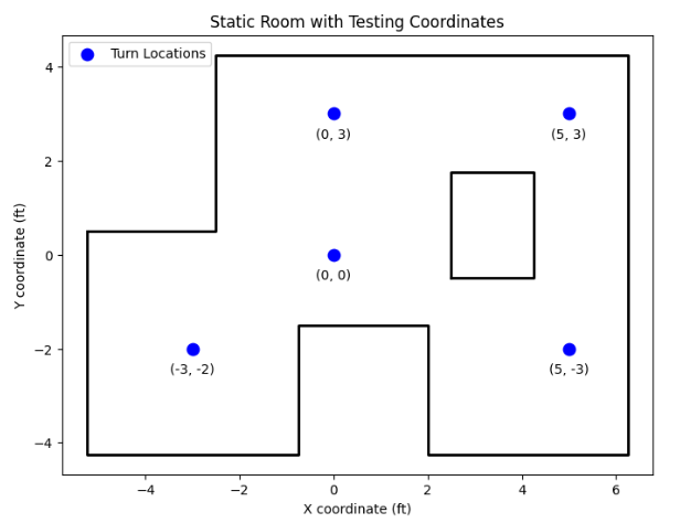
After the optimized tuning, I was able to test my robot in the lab space. The static room in the lab can be mapped out as the following diagram below. The diagram also denotes the points in which I took the measurements, the four points indicated in the lab handout, (-3,-2), (5, 3), (5, -3), (0, 3), and the origin (0, 0) in which I also took measurements for a better reference of the overall image of the room.
Here is an example of my system while it was untuned, at (-3,-2) coordinates. While it was untuned, it took shorter time to rotate, however, would send faulty and noisy measurements (check the bloopers section at the end for reference!).
For reference of my robot's performance, below is a video showing my robot's mapping performance at the mapped location (5, -3). This is an example of a tuned system. The system was able to measure yaw values very accurately, as well as the distance values at a very large range, but in order to do so, a longer period for reading the yaw value was implemented, increased to about 2000 ms. (The video is slightly sped up due to uploading issues.)
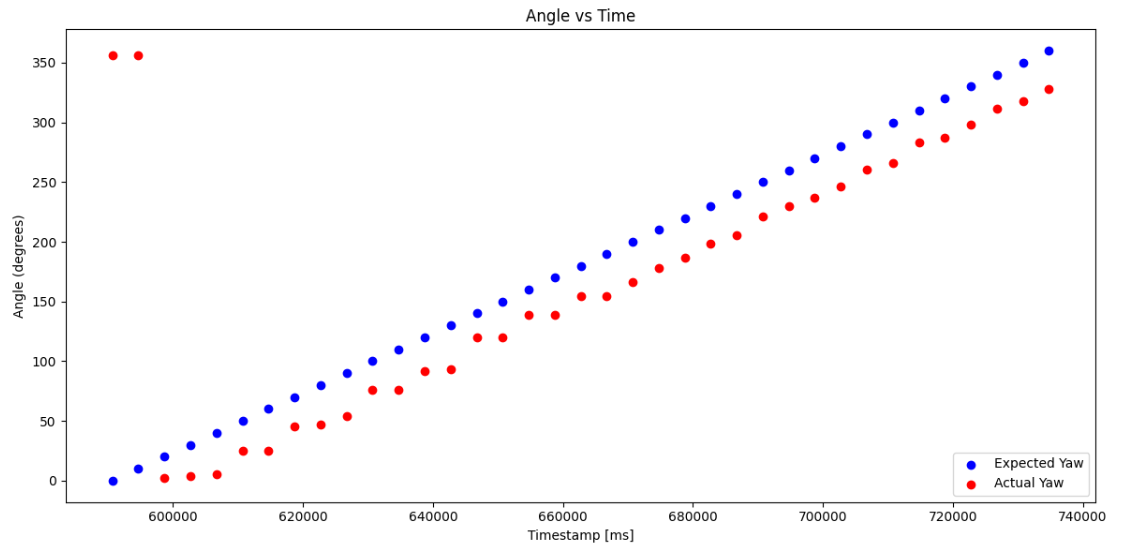
Analyzing the data arrays that were sent over Bluetooth, I was able to confirm the accuracy of my measurements through plotting the actual yaw values and the expected yaw values over the time they were recorded. The plot once the system was tuned looked like the following:
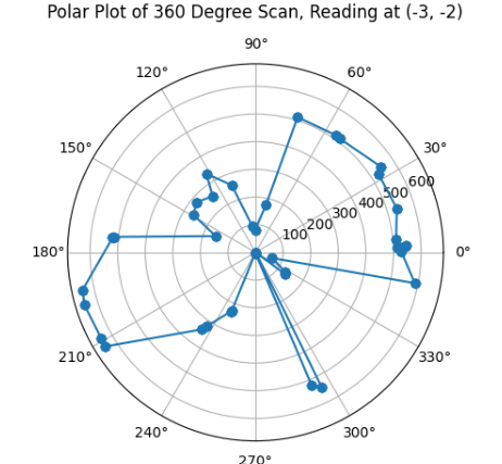
Afterwards, I determined the polar plots for each of the coordinate's datasets. The code attached below represents the code used for all attached polar plots. I took the advice proposed in the handout about maintaining the starting position of the robot in all testing coordinates constant, hence I pointed my robot along the positive x-axis and rotated clockwise 360 degrees. Furthermore, I determined that there was a distance between the robot's center of rotation and my used ToF sensor of about 7.5 cm, which was accounted for as the pre-processing on the data in order to obtain more accurate measurements of the mapping when determining the polar plots.
global radians

neg_actual_yaw = [x for x in actual_yaw]
radians = np.radians(neg_actual_yaw)
plt.figure()
ax = plt.subplot(111, polar=True)
ax.plot(radians[0:37], tof_distance[0:37], marker='o')

# Set angle ticks (degrees)
ax.set_thetagrids(np.arange(0, 360, 30), fontsize = 10)  # Set tick marks every 45°
ax.set_theta_direction(-1)

ax.set_title("Polar Plot of 360 Degree Scan, Reading at (5, 3)", va='bottom', pad = 30)
plt.show()
print(radians)
print(tof_distance)
print(actual_yaw)
With the code applied to all the datasets accumulated at each of the measuring coordinates, I was able to obtain the following polar plots:
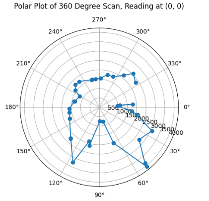
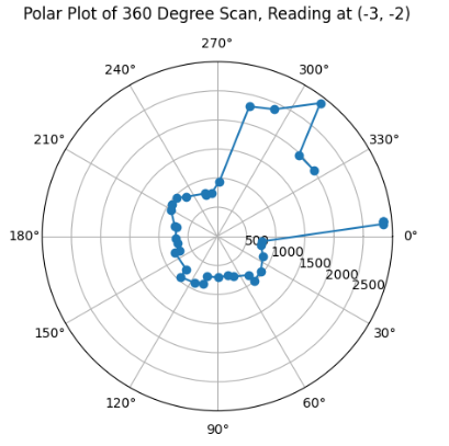
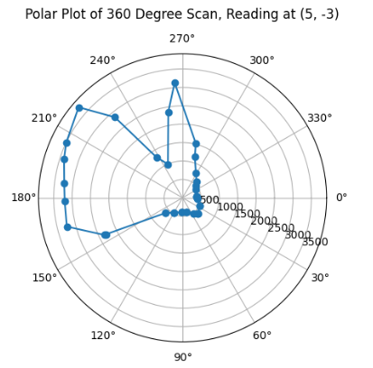
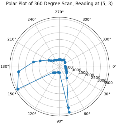
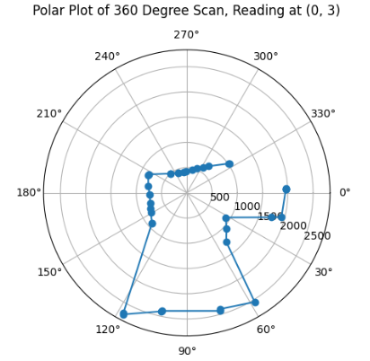
As can be inferred from my Polar Plots, since my robot's original positionality at every coordinate is in positive x-axis direction, then in my code for polar plots above, I implemented the following line ax.set_theta_direction(-1), which enabled the rotation of the measured angles to start at 0 at the positive x-axis direction, so that I am able to more easily visualise the view of my robot moving thorugh space at the set coordinate as if I am looking down at the coordinate. Furthermore, the data looks as expected through comparing it to previous year's lab pages, such as TA Daria Kot's (2024).
Merge and Plot Readings
Considering the aforementioned directionality of the robot initially at the origin, we can notice that with the particular orientation I chose, we can determine the transformation matrix from polar coordinates to Cartesian system. Hence, for the given measured angle value - theta value - we can predict the behaviour of the matrix as the following:
| angle - theta | x | y |
|---|---|---|
| 0 | 1 | 0 |
| 90 | 0 | -1 |
| 180 | -1 | 0 |
| 270 | 0 | 1 |
which effectivaly represents x = r * cos (θ), and y = -r * sin(θ). Based on that, the transformation matrix would look like the following:
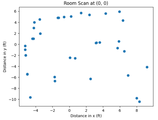
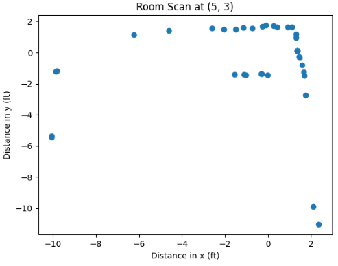
Based on that, we can make the following implementation to convert to Cartesian form in Python. This was performed for each of the datasets for every coordinate point. The example for coordinate of (5, 3) is provided below.
x_53 = []
y_53 = []

for i in range(len(radians[0:37])):
    x_53.append(tof_distance[i] * np.cos(radians[i]) / (2.54*12*10))
    y_53.append(-1.0 * tof_distance[i] * np.sin(radians[i]) / (2.54*12*10))

plt.figure()
plt.scatter(x_53, y_53, marker='o')
plt.xlabel('Distance in x (ft)')
plt.ylabel('Distance in y (ft)')
plt.title('Room Scan at (5, 3)')
plt.show()
As can be inferred from the code, there is a conversion implemented on the appended value to the two arrays, since values on the polar plot were expressed in milimeters (hence inches * feet * milimeters conversion). Afterwards, I was able to obtain plots for each of the coordinate points.
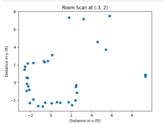
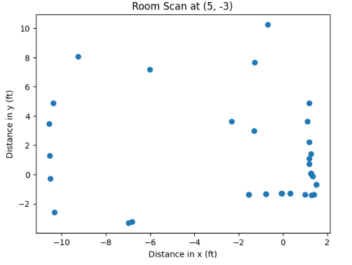
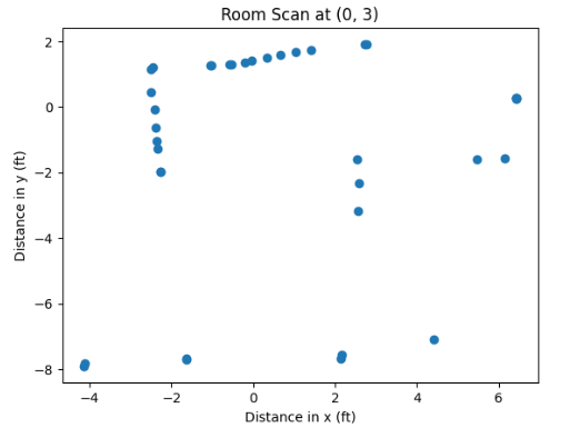
However, these Cartesian systems are relative, and do not quite fit into the global perspective of the Cartesian system relative to (0,0) reading. Hence, we ought to add the coordinates of the rotation center from which the points were taken to each of the obtained and stored pairs of x and y. This can be performed through manipulating and translating the array sets in Python as the following:
# (0, 0)
x_00_global = np.array(x_00)
y_00_global = np.array(y_00)

# (5, 3)
x_53_global = np.array(x_53) + 5.0
y_53_global = np.array(y_53) + 3.0

# (5, -3)
x_5_neg3_global = np.array(x_5_neg3) + 5.0
y_5_neg3_global = np.array(y_5_neg3) - 3.0

# (0, 3)
x_03_global = np.array(x_03)
y_03_global = np.array(y_03) + 3.0

# (-3, -2)
x_32_global = np.array(x_32) - 3.0
y_32_global = np.array(y_32) - 2.0

plt.figure()
plt.scatter(x_32_global, y_32_global, c='g', marker='o')
plt.scatter(x_53_global, y_53_global, c='b', marker='o')
plt.scatter(x_03_global, y_03_global, c='r', marker='o')
plt.scatter(x_5_neg3_global, y_5_neg3_global, c='m', marker='o')
plt.scatter(x_00_global, y_00_global, c='c', marker='o')
plt.scatter([-3, 5, 0, 5], [-2, 3, 3, -3], c='b', marker='x', label='Turn Locations')
plt.xlabel('X coordinate (ft)')
plt.ylabel('Y coordinate (ft)')
plt.title('Merged Mapped Space Without Lines')
plt.show()
Running the attached code after performing the translation of our obtained arrays, we ought to obtain something like the following.
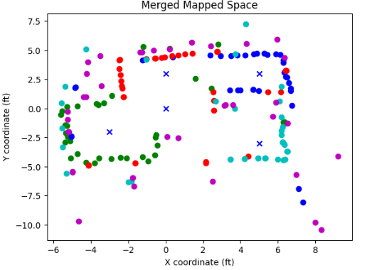
As can be inferred from the image, the captured distances ad the trend of the static room are clearly detectable, with the square-shaped box in the upper-right corner well detected. Through experimentation, I determined the coordinates which represent the walls of the room, and added them to my proposed plot of the global space.
wall_x = [-5.25, -5.25, -0.75, -0.75, 0.75, 2, 6.25, 6.25, -2.5, -2.5, -5.2]
wall_y = [0.5, -4.25, -4.25, -2.5, -2.5, -4.5, -4.5, 4.5, 4.5, 0.5, 0.5]
box_x = [2.5, 4.25, 4.25, 2.5, 2.5]
box_y = [-0.5, -0.5, 1.75, 1.75, -0.5]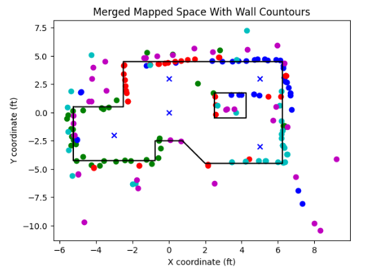
Finally, cleaning up the distances that are far away from the contours through code, we ought to obtain something similar to the following:
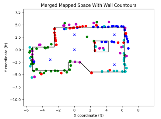
As can be inferred, the proposed mapped global map is able to detect the contours of the proposed static room very accurately relative to the four points. We ought to convert the lists into the lists of the form (x_start, y_start), and (x_end, y_end) as was noted in the manual. Below is the attached code for doing so, as well as the outputted lists:
wall_start = []
wall_end = []
box_start = []
box_end = []
for i in range(len(wall_x) - 1):
    wall_start += [[wall_x[i], wall_y[i]]]
    wall_end += [[wall_x[i+1], wall_y[i+1]]]
for i in range(len(box_x) - 1):
    box_start += [[box_x[i], box_y[i]]]
    box_end += [[box_x[i+1], box_y[i+1]]]
[[-5.25, 0.5], [-5.25, -4.25], [-0.75, -4.25], [-0.75, -2.5], [0.75, -2.5], [2, -4.5], [6.25, -4.5], [6.25, 4.5], [-2.5, 4.5], [-2.5, 0.5]] # wall_start
[[-5.25, -4.25], [-0.75, -4.25], [-0.75, -2.5], [0.75, -2.5], [2, -4.5], [6.25, -4.5], [6.25, 4.5], [-2.5, 4.5], [-2.5, 0.5], [-5.2, 0.5]] # wall_end
[[2.5, -0.5], [4.25, -0.5], [4.25, 1.75], [2.5, 1.75]] # box_start
[[4.25, -0.5], [4.25, 1.75], [2.5, 1.75], [2.5, -0.5]] # box_end
Bloopers - kind of
While testing my robot and plotting my data, since my sensor was very noisy, and through reading the Example1_readDistance script from SparkFun VL53L1X 4m Laser Distance Sensor examples, I realized with TA Cameron that my measurements were very fault and that my sensor would not read distances above 200 mm. The ultimate fix was changing the timing budget to 200 ms, as proposed earlier, but mostly resoldering the connections. However, even though noisy and faulty, the sensors produces interesting images on the polar plots.
Discussion
This lab was one of the most interesting labs in my opinion, it presents us with a new chapter into localization and planning, as well as incorporates the knowledge obtained in many previous labs, fundamentally Lab 6.
Acknowledgements and References
*I worked with Becky Lee on this lab, and Ben Liao who helped me with understanding conversion to global frame. I referenced Ben Liao's website (2025) since I got help from him, as well as Wenyi Fu's website (2024) in order to understand the material better. Apart from the Becky and Ben, thank you to TA Cameron for helping me fix my ToF sensor connections, as well as TA Cheney for generously prolonging his office hours for testing purposes.