LAB 10

Localization

Localization represents a process in which our robot uses the information about its surrounding based on probability in order to infer its position, due to the fact that it does not have the "true" knowledge of its position. In order to implement localization, we develop the Bayes Filter on our robot, which operates on a "belief" - which is influenced by sensor measurements and control inputs, allowing the robot to make a prediction of its position in space. With the sensor measurements and control inputs updating, the robot ought to update its belief as well due to the Bayesian interference. The state of the robot is represented in x and y coordinates, where x coordinates were defined the same as in Lab 9, -5.5 ft < x < 6.5 ft, and y coordinates were defined the same as in Lab 9, -4.5 ft < y < 4.5 ft. Furthermore, the orientation of the robot can be described as the following: - 180 degrees < θ < 180 degrees.

The 3D space around the robot is discretized into a grid of the volume of 12x9x9 cells, where each of the cells can be represented in 1x1 ft of planar space and 20 degrees of orientation.

Bayes Filter Algorithm Implementation

Bayes Filter is a probabilistic algorithm used for estimating state of a dynamic system given observations, by leveraging Bayesian inference, through which it constantly updates beliefs about the state based on updated sensor measurements and control inputs. The prediction step of the Filter increases the belief uncertainty, while the update step decreases the belief uncertainty. The algorithm was presented to us in class Lecture 20, and can be described by the following figure:

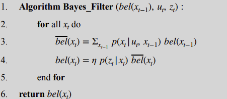Bayes Filter Algorithm

From the figure above, it can be inferred that \(bel(x_{t-1})\) represents the previous belief, which can be described as a 3D matrix, where each element further represents the probability that the robot is located in the compatible grid vell. Furthermore, \(u_{t}\) represents the current control input changing the pose from \(x_{t-1}\) to \(x_{t}\), while \(z_{t}\) represents the current sensor rate of 18 readings with 20 degree increments. The algorithm performs through looping through the range of \(x_{t}\) values, described in the form of (\(x, y, θ\)) at each point in time. Hence, new belief with each iteration is determined, through multiplying the new state's probability with the previous state's probability, resulting into the sum of all multiplications represented in the prediction belief \( \overline{\mathrm{bel}}(x_t) \). The belief is thus updated by multiplying the probability of new sensor readings at the current pose and performing the normalization with η after which \( {\mathrm{bel}}(x_t) \) is obtained and returned.

The figure below represents the odometry model parameters, which can be used to describe the control inputs, as follows from Lecture 18 on Bayes Filter.. The odometry model represents the difference between two poses of the robot as initial rotation, translation, as well as final rotation.

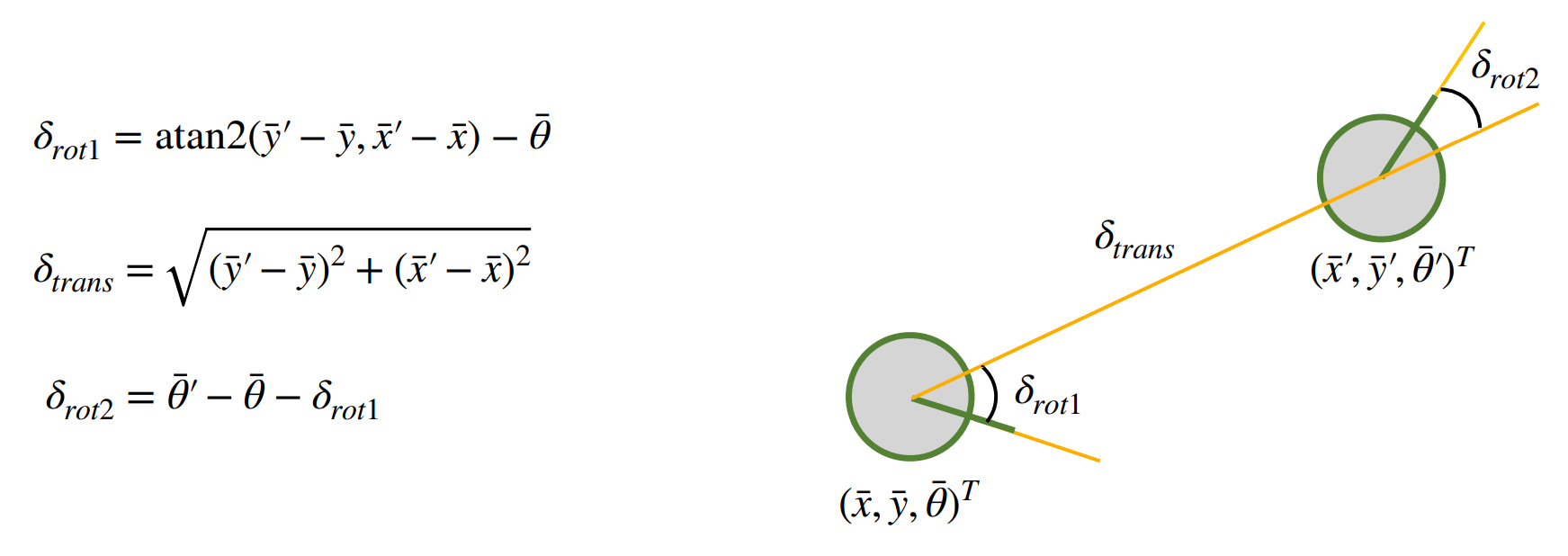Odometry Model Parameters

Compute Control

As aforementioned, the odometry model is computed through taking the difference between the previous and the current pose of the robot, and hence determining the initial rotation, translation, and final rotation, as in the formulas described in the Odometry Model Parameters figure above. This can be determined through NumPy's arctan2() function. The rotations are normalized to [-180, 180], and are calculated, as well as the translation.

def compute_control(cur_pose, prev_pose):
    """ Given the current and previous odometry poses, this function extracts
    the control information based on the odometry motion model.

    Args:
        cur_pose  ([Pose]): Current Pose
        prev_pose ([Pose]): Previous Pose 

    Returns:
        [delta_rot_1]: Rotation 1  (degrees)
        [delta_trans]: Translation (meters)
        [delta_rot_2]: Rotation 2  (degrees)
    """
    y_comp = cur_pose[1] - prev_pose[1]
    x_comp = cur_pose[0] - prev_pose[0]
    theta_prev = prev_pose[2]
    theta_cur = cur_pose[2]
    delta_1 = np.degrees(math.atan2(y_comp, x_comp)) - theta_prev
    delta_rot_1 = mapper.normalize_angle(delta_1)
    delta_trans = math.sqrt(y_comp**2+x_comp**2)
    delta_rot_2 = mapper.normalize_angle(theta_cur - theta_prev - delta_1)

    return delta_rot_1, delta_trans, delta_rot_2  

Odometry Motion Model

The odometry motion model is responsible for the probability that the motion calculated in the previous step was performed. This is performed by taking the previous pose and the current pose through odom_motion_model(), and extracting the odometry model parameters from them using compute_control(), calculating the probabilities of the parameters. Hence, the inputs consist of the current pose, previous pose, and odometry control values (u) for rotation_1, rotation_2, and translation. Knowing the current position as well as the previous position, the odometry control values (u), the return value is the probability p(x'|x,u)that the robot achieved the current position x'. The Gaussian distribution can be examined, while each of the events can be represented as independent. The probability of each of the events is thus multiplied in order to obtain the motion probability.

def odom_motion_model(cur_pose, prev_pose, u):
    """ Odometry Motion Model

    Args:
        cur_pose  ([Pose]): Current Pose
        prev_pose ([Pose]): Previous Pose
        (rot1, trans, rot2) (float, float, float): A tuple with control data in the format 
                                                    format (rot1, trans, rot2) with units (degrees, meters, degrees)


    Returns:
        prob [float]: Probability p(x'|x, u)
    """

    u_calc = compute_control(cur_pose, prev_pose)
    rot1_x = mapper.normalize_angle(u_calc[0])
    rot1_mu = mapper.normalize_angle(u[0])
    trans1_x = u_calc[1]
    trans1_mu = u[1]
    rot2_x = mapper.normalize_angle(u_calc[2])
    rot2_mu = mapper.normalize_angle(u[2])
    rot1_prob = loc.gaussian(mapper.normalize_angle(rot1_x-rot1_mu), 0, loc.odom_rot_sigma)
    trans_prob = loc.gaussian((trans1_x-trans1_mu), 0, loc.odom_trans_sigma)
    rot2_prob = loc.gaussian(mapper.normalize_angle(rot2_x - rot2_mu), 0, loc.odom_rot_sigma)

    prob = rot1_prob * trans_prob * rot2_prob

    return prob

Prediction Step

The prediction step utilized 6 nested loops in order to calculate the probability of the robot moving onto the next grid cell. The inputs are the previous odometry position (prev_odom), as well as the current odometry position (cur_odom). The if statement speeds up the Filter, with the statement checking for the belief greater than 0.0001. If the belief is less than the value, then the code does not proceed with the remaining three for loops, due to the fact that the robot's position is not likely to be in those remaining grid cells. However, if the belief fulfills the greater or equal to condition, then the probability is calculated.

def prediction_step(cur_odom, prev_odom):
    """ Prediction step of the Bayes Filter.
    Update the probabilities in loc.bel_bar based on loc.bel from the previous time step and the odometry motion model.

    Args:
        cur_odom  ([Pose]): Current Pose
        prev_odom ([Pose]): Previous Pose
    """

    u = compute_control(cur_odom, prev_odom)
    for prev_x in range(mapper.MAX_CELLS_X):
        for prev_y in range(mapper.MAX_CELLS_X-3):
            for prev_a in range(mapper.MAX_CELLS_A):
                if loc.bel[prev_x,prev_y,prev_a] >= 0.0001:
                    for cur_x in range(mapper.MAX_CELLS_X):
                        for cur_y in range(mapper.MAX_CELLS_Y):
                            for cur_a in range(mapper.MAX_CELLS_A):
                                prev_pose = mapper.from_map(prev_x,prev_y,prev_a)
                                current_pose = mapper.from_map(cur_x,cur_y,cur_a)
                                prob = odom_motion_model(current_pose,prev_pose,u)
                                bel = loc.bel[prev_x-1,prev_y-1,prev_a-1]
                                loc.bel_bar[cur_x,cur_y,cur_a] += (prob*bel) 

Sensor model

The sensor model step is based on finding the probability of the sensor measurements, which are modeled as the Gaussian distribution. The value of 18 represents the 18 different distance readings. The input is represented in the one-dimensional observation array obs for the pose of the robot. The returned array is represented in the same one-dimensional array with the likelihood of each of the events prob_array.

def sensor_model(obs):
    """ This is the equivalent of p(z|x).


    Args:
        obs ([ndarray]): A 1D array consisting of the true observations for a specific robot pose in the map 

    Returns:
        [ndarray]: Returns a 1D array of size 18 (=loc.OBS_PER_CELL) with the likelihoods of each individual sensor measurement
    """
    prob_array = np.zeros(18)
    for i in range(18):
        prob_array[i] = loc.gaussian(loc.obs_range_data[i], obs[i], loc.sensor_sigma)

    return prob_array 

Update Step

The update step represents the belief of the robot per grid cell. Hence, the probability (p(z|x))is multiplied by the predicted belief loc.bel_bar to obtain loc.bel, or the belief, which is further normalized.

def update_step():
    """ Update step of the Bayes Filter.
    Update the probabilities in loc.bel based on loc.bel_bar and the sensor model.
    """
    for cur_x in range(mapper.MAX_CELLS_X):
        for cur_y in range(mapper.MAX_CELLS_Y):
            for cur_a in range(mapper.MAX_CELLS_A):
                prob = np.prod(sensor_model(mapper.get_views(cur_x,cur_y,cur_a)))
                loc.bel[cur_x,cur_y,cur_a] = loc.bel_bar[cur_x,cur_y,cur_a] * prob
    loc.bel = loc.bel / np.sum(loc.bel)

Results

The following video represents the trajectory simulation without the Bayes filter. The deterministic odometry model is plotted in red, while the ground truth is represented in green. As can be inferred from the video, the odometry model is not very reliable.

The following video represents adding the Bayes Filter to the localization simulation. With this simulation, we have the probabilistic belief indicated in blue, which has a close accuracy in approximation of the robot's true position. The probabilistic approach reflects the sensor data being more consistent and trustworthy when it is oriented around the walls, and less trustworthy in larger unconstrained spaces, causing larger errors as can be seen from the raw data .txt file below. The probabilistic belief can be seen to follow the ground truth plotted in green pretty well, while the odometry model represented in red still has a non-reliable trajectory.

The raw data collected can be found here: Raw data collected from the run

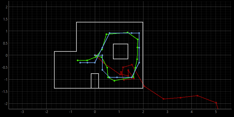Localization with Bayes Filter example 1

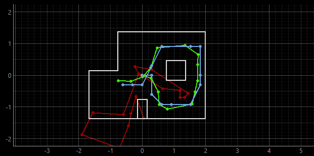Localization with Bayes Filter example 2